Bode plot
A Bode plot is a graphical representation of a closed-loop system's loop-gain LG(s) frequency response. It is a widely used tool in control systems engineering, electronics, and signal processing to analyze and design closed-loop linear time-invariant (LTI) systems. Bode plots provide insights into how a system responds to different frequencies, helping engineers understand its stability, gain, and phase characteristics.
Free online Bode plot generator
Components of a bode plot (Frequency, Magnitude and Phase)
There are three components of a bode plot, namely frequency, magnitude of the transfer function, and phase of the transfer function.
Frequency (x-axis or ω)
The horizontal axis of a Bode plot represents the frequency of the input signal. Frequencies are typically plotted on a logarithmic scale, usually in decades (powers of 10) or octaves (doubling of frequency). Decades scale is the most popular.
Magnitude (y-axis or dB)
The vertical axis represents the magnitude (amplitude) of the system's response. The magnitude is often expressed in decibels (dB). The magnitude plot shows how the system amplifies or attenuates signals at different frequencies. It is plotted on a logarithmic scale. It means both the x-axis and y-axis are plotted in a logarithmic scale.
$$y=20log{}_{10}(|LG(j\omega{})|)$$
Phase (y-axis or °)
The phase plot represents the phase shift introduced by the system at different frequencies. Phase is typically measured in degrees or radians. It shows the time delay or advance of the output signal relative to the input signal at each frequency. It is plotted on a semilog scale. It means that the x-axis (frequency) is plotted on a logarithmic scale while the y-axis is plotted on a linear scale.
$$y=\angle{}LG(j\omega{})$$
How to draw a bode a plot ?
If a transfer function is provided, it is important to convert the transfer function into a standard (bode-friendly) form. This is done to identify the poles, zeros, and low-frequency magnitude of function correctly.
Numerical tools like Python (Scipy) and MATLAB can always be used to generate very accurate bode plots but hand-drawn plot allows us to understand the function better.
For example -
$$H(s)=3000\cfrac{s+10}{(s+3)(s+100)}$$
We need to convert the above equation into bode-friendly form :
$$H(s)=100\cfrac{s/10+1}{(s/3+1)(s/100+1)}$$
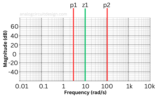
The above equation has 2 poles and 1 zero. We should mark the frequencies of poles and zeros in the x-axis of the bode plot. The magnitude is converted into dB by using the 20log10(Magnitude) formula.
Identify poles and zeros
In the above equation, the poles are :
$$p_1=3$$
$$p_2=100$$
and zeros are :
$$z_1=10$$
Please note that the bode plot's x-axis never starts from 0. It starts from a very low frequency.
Find the DC / Low frequency magnitude
To start the bode plot we need to obtain the magnitude of the function at a convenient frequency. We chose DC/low-frequency to be a convenient po\int.
If we substitute s=0 in the above equation, we obtain a magnitude of 100. We need to convert this into dB in the following way:
$$\text{Magnitude}=20\log{}_{10}\left(100\right)=40\,\text{dB}$$
Traversing through poles and zeros in the graph, intuitively
We shall make separate Magnitude and Phase plots :
Magnitude plot
Whenever we pass through a pole, the graph line will fall at the rate of -20dB/decade. Whenever we pass through a zero, the graph line will increase at the rate of +20dB/decade. To understand this, we see the equation H(s), where the zero is trying to increase the magnitude of the function while the poles are decreasing the magnitude. The rates of 20dB/decade are asymptotic, which means the actual graph will show a 20dB/decade rate not immediately after the pole/zero is passed.
To intuitively understand the procedure, we can rewrite the transfer function as :

We have arranged the factors in the expression such that the lowest frequency pole/zero is at the left and the highest frequency pole/zero is at the \right.
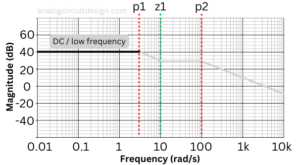
In the above figure, the low frequency is plotted. In the transfer function, we replace s with a very low-frequency value. The magnitude is represented in dB.
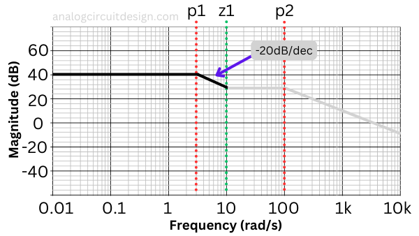
After the first pole is hit, the magnitude in the transfer function starts dropping by -20dB/decade. It means a 10x drop in magnitude for a 10x increase in frequency. We should note that at the frequency of the pole, the magnitude is 1/√2 (= -3dB). However, this error is neglected in the asymptotic bode plot which we are drawing.
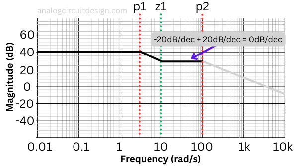
After the zero is hit, whatever magnitude loss we were facing due to the pole is compensated by the increase in magnitude due to the zero. That is why the magnitude curve remains flat. It will settle at value :
$$H(10<s<100)=100\cfrac{3}{10}=30$$
$$20\log{}_{10}(30)=29.5\,\text{dB}$$
So, between the frequency range of 10rad/s to 100rad/s, the plot will have a magnitude of 29.5dB.
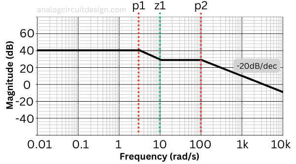
After the flat region, we again arrive at a pole. So, 2 poles will overwhelm the one and only zero and the plot will start dropping at -20dB/decade.
Phase plot
While making a phase plot, it is helpful to mark the pole and zero location. Since we do not have any pole/zero at origin (0), we do not lose or gain phase at origin. So, our phase starts at 0°.
Whenever we reach a pole frequency, we must lose 45° at exactly the pole frequency. A decade earlier (0.1 times) of the pole frequency we must have lost 5° and a decade later (10 times) of the pole frequency, we must lose 85°. We can neglect 5° or 85° for hand-drawn bode plots and replace these numbers with 0° and 90° respectively for simplicity.
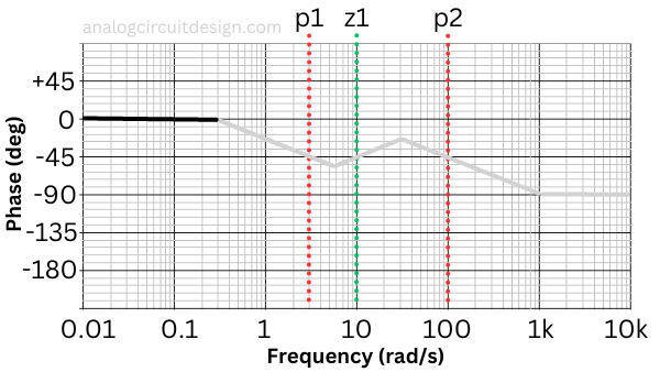
There is no phase loss/gain initially at low frequency because we have not crossed any pole/zero. So, the starting phase is 0°.
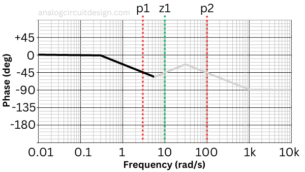
The phase loss at the frequency of the pole is 45°. The phase starts dropping a decade before the pole appears. So, in this case, the phase starts dropping from 0.3rad/sec (which is a decade before 3rad/sec). At 3rad/sec, the phase is -45°. This comes from the fact that at pole frequency ( ω = p1 ), phase (φ) is given by :
$$\phi{}=-tan{}^{-1}\left(\cfrac{\omega{}}{p_1}\right)=-45^o$$
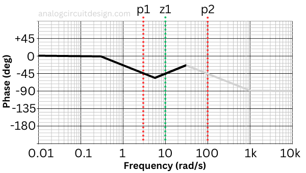
After the zero is hit, the phase starts increasing. At the frequency of zero, if the system has only zero, the phase is $45^o$. $$\phi{}=tan{}^{-1}\left(\cfrac{\omega{}}{z_1}\right)=45^o$$
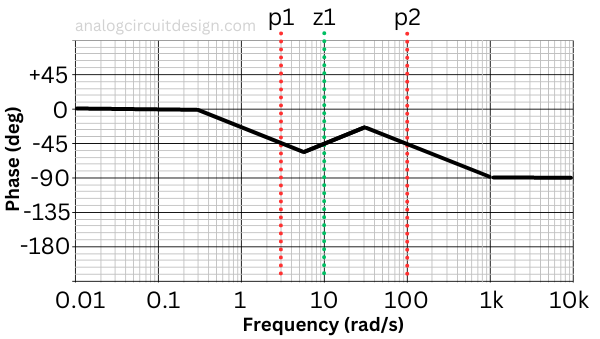
After the last pole is hit, the phase starts decreasing again. The phase due to the previous pole and zero was canceled. Only the last pole is left. So, again it would be -45° at p2. At higher frequencies, since there is no more pole or zero, the phase dropped and saturated to -90°.
For higher frequency (ω > p2),
$$\phi{}=-tan{}^{-1}\left(\cfrac{\omega{}}{z_1}\right)=-90^o$$
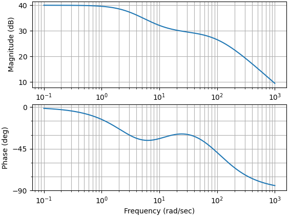
Exact bode plot of the transfer function using Python
Using a Python computer program, we can plot the exact bode plot of a transfer function. The exact bode plot of the transfer function H(s) is mentioned below. We can use MATLAB too.
    import numpy as np
    import control.matlab as ml
    num=np.array([100/10,100])
    den=np.polymul(np.array([1/3,1]),np.array([1/100,1]))
    G=ml.tf(num,den)
    print(ml.pole(G))
    import matplotlib.pyplot as plt
    mag,phase,w=ml.bode(G)
    plt.show()
Matlab code to generate a bode plot

% Define numerator and denominator
num = [100/10 100];
den = conv([1/3 1], [1/100 1]); % convolution = polymul in Python

% Create transfer function
G = tf(num, den);

% Display poles
disp('Poles of G:');
disp(pole(G));

% Generate and plot Bode plot
figure;
bode(G);
grid on;
Application of bode plot
- Stability Analysis: Engineers can determine the stability of a system by examining the magnitude and phase plots. A system is considered stable if its phase margin is positive and its gain margin is greater than 0 dB.
- Frequency Response Analysis: Bode plots allow engineers to understand how a system responds to different frequencies. For example, they can determine the system's bandwidth, resonance frequency, and the frequency at which phase shift becomes critical.
- Design and Tuning: Engineers can use Bode plots to design and tune control systems. By adjusting the system's parameters, they can achieve desired performance characteristics based on the Bode plot analysis.
Advantages of bode plot
- This approach relies on asymptotic approximations, offering a straightforward means to generate a logarithmic magnitude curve.
- When dealing with the transfer function, the multiplication of different magnitudes can be equated to addition, while division corresponds to subtraction when using a logarithmic scale.
- This graphical representation enables a quick assessment of system stability, removing the need for complex calculations.
- Bode plots furnish insights into relative stability through metrics like Gain margin and Phase margin, spanning a broad frequency spectrum from low to high frequencies.