Laplace transform
The Laplace transform converts integral and differential equations into algebraic equations allowing us to analyse complicated circuits having R, L and C. Important applications :
- Transfer functions
- Control systems
The Laplace transform
Laplace transform is valid for time \(t\geq{}0\). The Laplace transform of a signal (function) \(f\) is the function \(F=\mathcal{L}(f)\) defined by :
$$F(s)=\int_0^{\infty{}}f(t)e^{-st}dt$$
where,
$$s=\sigma{}+j\omega{}$$
\(s\) is called complex frequency variable with units sec-1. \(t\) is time (in seconds). \(F\) is a complex-valued function.
Basic examples of Laplace transforms
Laplace transform of \(f(t)=e^t\)
$$F(s)=\int_0^{\infty}e^te^{-st}dt=\int_0^{\infty}e^{(1-s)t}dt=\cfrac{1}{1-s}e^{(1-s)t}|_0^{\infty}=\cfrac{1}{s-1}$$ The above result is valid for \(Re(s)=\sigma{}\geq{}1\). Otherwise \(F(s)\) it is non-convergent function.
Laplace transform of \(f(t)=u(t)\)
$$u(t)=1\hspace{1cm}t\geq{}0$$ $$u(t)=0\hspace{1cm}t<0$$
$$F(s)=\int_0^{\infty{}}e^{-st}dt=-\cfrac{1}{s}e^{-st}|_0^{\infty{}}=\cfrac{1}{s}$$ The above result is valid for \(Re(s)=\sigma{}\geq{}0\). Otherwise \(F(s)\) it is non-convergent function.
Laplace transform of \(f(t)=t^n\hspace{0.5cm}(n\geq{}1)\)
Using integrate by parts,
$$\int_a^bu(t)v'(t)dt=u(t)v(t)|_a^b-\int_a^bv(t)u'(t)dt$$
where \(u(t)=t^n,v'(t)=e^{-st},a=0,b=\infty{}\)
$$F(s)=\int_0^{\infty}t^ne^{-st}dt=t^n\left(\cfrac{-e^{-st}}{s}\right)|_0^{\infty}+\cfrac{n}{s}\int_0^{\infty}t^{n-1}e^{-st}dt$$ $$F(s)=\cfrac{n!}{s^{n+1}}$$
Laplace transform of impulse function \(\delta{}(t)\)
If \(f\) contains impulse at t=0, it can be included in the integral by defining F:
$$F(s)=\int_{0^-}^{\infty}f(t)e^{-st}dt$$
Impulse function \(\delta{}(t)\)
$$F(s)=\int_{0^-}^{\infty}\delta{}(t)e^{-st}dt=e^{-st}|_{t=0}=1$$
Laplace transform of derivative of impulse function \(d^k\delta{}(t)/dt^k\)
$$F(s)=\int_{0^-}^{\infty}\cfrac{d^k\delta{}(t)}{dt^k}e^{-st}dt=(-1)^k\cfrac{d^k}{dt^k}e^{-st}|_{t=0}=s^ke^{-st}|_{t=0}=s^k$$
Basic properties of Laplace transform
Linearity
The Laplace transform in linear means principle of homogenity and superposition holds. If \(f\) and \(g\) are any signals and \(a\) is any scalar :
$$\mathcal{L}(af)=a\mathcal{L}(f)$$
$$\mathcal{L}(f+g)=\mathcal{L}(f)+\mathcal{L}(g)$$
Example
$$\mathcal{L}(5\delta{}(t)-3e^{-t})=5\mathcal{L}(\delta{}(t))-3\mathcal{L}(e^{-t})$$ $$=5-\cfrac{3}{s+1}$$ $$=\cfrac{5s+2}{s+1}$$
One to One property
The Laplace transform is one-to-one : if \(\mathcal{L}(f)=\mathcal{L}(g)\) then \(f=g\)
Example
There exist no other function \(f(t)\) $$f(t)=5\delta{}(t)-3e^{-t}$$ such that $$F(s)=\mathcal{L}(f)=\cfrac{5s+2}{s+1}$$
Time scaling
If \(g(t)=f(at)\) where \(a > 0\); then
$$G(s)=\cfrac{1}{a}F(s/a)$$
Derivation
$$G(s)=\int_{0}^{\infty{}}f(at)e^{-st}dt=\cfrac{1}{a}\int_0^{\infty}f(\tau)e^{-(s/a)\tau{}}d\tau{}=\cfrac{1}{a}F\left(\cfrac{1}{a}\right)$$
Exponential scaling
If \(g(t)=e^{at}f(t)\) then
$$G(s)=F(s-a)$$
Derivation
$$G(s)=\int_{0}^{\infty{}}e^{-st}e^{at}f(t)dt=\int_{0}^{\infty}e^{-(s-a)t}f(t)dt=F(s-a)$$
Time delay
Let \(f\) be a signal and \(T>0\); define signal \(g\) as
$$g(t)=\begin{cases}0 & 0\leq{}t<T \\\ f(t-T) & t\geq{}T\end{cases}$$
Function \(g\) is delayed \(f\) by \(T\) seconds and zero-padded up to \(T\).
$$G(s)=e^{-sT}F(s)$$
Derivation
$$G(s)=\int_0^{\infty}e^{-st}g(t)dt=\int_T^{\infty}e^{-sT}f(t-T)dt=\int_0^{\infty}e^{s(\tau{}+T)}f(\tau{})d\tau{}=e^{-sT}F(s)$$
Derivative
If signal \(f\) is continuous at \(t = 0\), then
$$\mathcal{L}(f')=sF(s)-f(0)$$
- Time-domain differentiation becomes multiplication by frequency variable "\(s\)".
- Additional a term called intial condition is added i.e., \(f(0)\)
For higher-order derivates,
$$\mathcal{L}(f'')=s\mathcal{L}(f'')-f'(0)$$ $$=s(sF(s)-f(0))-f'(0)$$ $$=s^2F(s)-sf(0)-f'(0)$$
Example
Laplace transform of impulse function \(\delta{}(t)\). Impulse function is derivative of unit step function \(u(t)\). Laplace transform of unit step function is derived earlier. $$f'(t)=\delta{(t)}$$ $$\mathcal{L}(f')=s\left(\cfrac{1}{s}\right)-0=1$$
A general expression of Laplace transform of derivates :
$$\mathcal{L}\left(\cfrac{df^n(t)}{dt^n}\right)=s^nF(s)-s^{n-1}f(0^-)-s^{n-2}\cfrac{df(0^-)}{dt}-\dots{}-s\cfrac{d^{n-2}f(0^-)}{dt^{n-2}}-\cfrac{d^{n-1}f(0^-)}{dt^{n-1}}$$
Integral
Let \(g\) be the running integral of a signal \(f(t)\) i.e.,
$$g(t)=\int_{-\infty{}}^tf(\tau{})d\tau{}$$
then,
$$G(s)=\cfrac{F(s)}{s}+\underbrace{\cfrac{\int_{-\infty{}}^{0}f(x)dx}{s}}_{\text{initial condition}}$$
Without initial condition,
$$G(s)=\cfrac{F(s)}{s}$$
Derivation
$$G(s)=\int_{t=0}^{\infty{}}\left(\int_{\tau{}=0}^{t}f(\tau{})d\tau{}\right)e^{-st}dt=\int_{t=0}^{\infty{}}\int_{\tau{}=0}^{t}f(\tau{})e^{-st}d\tau{}dt=\int_{t=0}^{\infty{}}f(\tau{})\left(\int_{\tau{}=0}^{t}e^{-st}dt\right)d\tau{}=\int_{t=0}^{\infty{}}f(\tau{})\cfrac{1}{s}e^{-s\tau{}}d\tau{}=\cfrac{F(s)}{s}$$
Multiplication by t
Let \(f(t)\) be a signal and define
$$g(t)=tf(t)$$ $$G(s)=-F'(s)$$
Derivation
$$F(s)=\int_0^{\infty{}}e^{-st}f(t)dt$$ with respect to \(s\) to get $$F'(s)=\int_0^{\infty}(-t)e^{-st}f(t)dt$$ or $$-F'(s)=\int_0^{\infty}tf(t)e^{-st}dt$$
Convolution
The convolution of signals \(f\) and \(g\), denoted \(h=f*g\) is the signal
$$h(t)=\int_0^{t}f(\tau{})g(t-\tau{})d\tau{}$$
same as
$$h(t)=\int_0^{t}f(t-\tau{})g(\tau{})d\tau{}$$
In other words, the relation between \(f\) and \(g\) is commutative
$$ f*g=g*f $$
Also,
$$H(s)=F(s)G(s)$$
Derivation
$$H(s)=\mathcal{L}(f*g)=F(s)G(s)$$ $$H(s)=\int_0^{\infty}e^{-st}\left(\int_{\tau{}=0}^tf(\tau{})g(t-\tau{})d\tau{}\right)dt$$ $$=\int_0^{\infty}\int_{\tau{}=0}^te^{-st}f(\tau{})g(t-\tau{})d\tau{}dt$$ Changing order of integration $$H(s)=\int_{\tau{}=0}^{\infty}\int_{t=\tau{}}^{\infty}e^{-st}f(\tau{})g(t-\tau{})dtd\tau{}$$ Change variable to \(\bar{t}=t-\tau{}, d\bar{t}=dt\) $$H(s)=\int_{\tau{}=0}^{\infty}\int_{\bar{t}=0}^{\infty}e^{-s(\bar{t}+\tau{})}f(\tau{})g(\bar{t})d\bar{t}d\tau{}$$ $$H(s)=\left(\int_{\tau{}=0}^{\infty}e^{-s\tau{}}f(\tau{})d\tau{}\right)\left(\int_{\bar{t}=0}^{\infty}e^{-s\bar{t}}g(\bar{t})d\bar{t}\right)$$
Inverse Laplace transform
In principle f(t) can be recovered from \(F(s)=\mathcal{L}(f(t))\) using :
$$f(t)=\cfrac{1}{2\pi{}j}\int_{\sigma-j\infty}^{\sigma+j\infty}F(s)e^{st}ds$$
where \(\sigma\) is large enough such that \(F(s)\) is defined for \(Re(s)\geq{}\sigma\). The above integral is called Bromwich integral.
More about inverse Laplace transform : Inverse Laplace transform.
Solving differential equations using Laplace transform
Example : Find the solution of following differential equation,
$$2\cfrac{d^2x(t)}{dt^2}+7\cfrac{dx(t)}{dt}+5x(t)=10u(t)$$
Initial conditions,
$$\cfrac{dx(0^-)}{dt}=1, x(0^-)=-2$$
Solution :
Taking Laplace transform on both the sides,
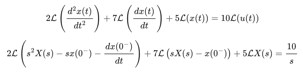
$$2\mathcal{L}\left(\cfrac{d^2x(t)}{dt^2}\right)+7\mathcal{L}\left(\cfrac{dx(t)}{dt}\right)+5\mathcal{L}(x(t))=10\mathcal{L}(u(t))$$
$$2\left(s^2X(s)-sx(0^-)-\cfrac{dx(0^-)}{dt}\right)+7\left(sX(s)-x(0^-)\right)+5X(s)=\cfrac{10}{s}$$
Substituting the initial conditions,
$$(2s^2+7s+5)X(s)=\cfrac{10}{s}-4s-12=\cfrac{10-4s^2-12s}{s}$$
Hence,
$$X(s)=\cfrac{-2s^2-6s+5}{s(s+2.5)(s+1)}$$
Now we need to start the process of inverse Laplace transform,
$$X(s)=\cfrac{K_1}{s}+\cfrac{K_2}{s+2.5}+\cfrac{K_3}{s+1}$$
After finding K1, K2 and K3,
$$X(s)=\cfrac{2}{s}+\cfrac{2}{s+2.5}-\cfrac{6}{s+1}$$
$$x(t)=\mathcal{L}^{-1}\left(\cfrac{2}{s}+\cfrac{2}{s+2.5}-\cfrac{6}{s+1}\right)$$ $$=(2+2e^{-2.5t}-6e^{-t})u(t)$$
Frequency domain analysis using Laplace domain
Frequency domain analysis in the Laplace domain involves representing a system’s behavior using the complex frequency variable \(s = \sigma{}+j\omega{}\). By transforming a system’s differential equations into algebraic equations through the Laplace transform, system properties such as stability, transient response, and steady-state behavior can be analyzed. The Laplace domain provides a generalized framework that includes both the exponential decay/growth factor \(\sigma{}\) and sinusoidal frequency \(\omega{}\), making it a powerful tool for studying system dynamics. For steady-state sinusoidal analysis, the Laplace domain reduces to the Fourier domain by setting \(\sigma{} = 0\), i.e., \(s = j\omega{}\)
Transfer function of filters
The transfer function of a filter is a mathematical representation of the relationship between the output and input of the filter in the Laplace domain. It is defined as: $$H(s)=\cfrac{Y(s)}{X(s)}$$
where X(s) is the Laplace transform of the input signal, Y(s) is the Laplace transform of the output signal, and \(s = \sigma{} + j\omega{}\).
The transfer function characterizes the filter’s frequency response, allowing analysis of how different frequency components of the input are attenuated or amplified. Key features derived from the transfer function include: 1. Poles and Zeros: Indicate system stability and frequency behavior. 2. Magnitude Response: Shows gain vs frequency. 3. Phase Response: Shows phase shift vs frequency. 4. Type of Filter: Low-pass, high-pass, band-pass, or band-stop, based on how the transfer function behaves with respect to frequency.
Impedance of capacitor and inductor
Capacitor
The voltage-current relationship of a capacitor is: $$i(t)=C\cfrac{dV}{dt}$$ Taking the Laplace transform: $$I(s)=CsV(s)-Cv(0)$$ Assuming zero initial voltage (\(v(0)=0\)), the impedance of the capacitor in the Laplace domain is: $$Z_c(s)=\cfrac{V(s)}{I(s)}=\cfrac{1}{sC}$$ Steady state frequency domain analysis, $$Z_c(j\omega{})=\cfrac{1}{j\omega{}C}$$ The impedance decreases with increase in frequency, acting as a short circuit at high frequency.
Inductor
The voltage-current relationship of an inductor is: $$v(t)=L\cfrac{di(t)}{dt}$$ Taking the Laplace transform: $$V(s)=LsI(s)-Li(0)$$ Assuming zero initial current (\(i(0)=0\)), the impedance of the inductor in the Laplace domain is: $$Z_L(s)=\cfrac{V(s)}{I(s)}=sL$$ In the frequency domain \(s=j\omega{}\), $$Z_L(j\omega{})=j\omega{}L$$
Laplace analysis using Verilog A
Verilog-A allows designers to model linear time-invariant (LTI) systems using transfer functions expressed directly in the s-domain. Instead of writing differential equations manually, Laplace operators such as laplace_nd() and laplace_zp() enable intuitive representation of filters, amplifiers, and control blocks based on their numerator-denominator or zero-pole forms. These functions are solver-friendly and support AC, transient, and stability simulations without introducing nonlinear complexities. By abstracting mathematical behavior into compact expressions, Laplace modeling improves simulation efficiency, enhances reusability, and enables accurate frequency-dependent responses in analog and mixed-signal circuit design.
More about Verilog A Laplace analysis - Verilog-A Laplace Transform Analysis