Constellation Diagram
The Constellation Diagram is a two-dimensional X-Y graphical representation of symbols in the I (in-phase) and Q (quadrature) plane. When viewed as a polar coordinate system, the position of each symbol in the I–Q plane represents its amplitude (radius) and phase (angle). Signal constellations allow us to visualize modulation schemes and, more importantly, the effect of nonidealities on them.
Two signals are said to be in “quadrature” when they are separated in phase by exactly 90°. Signals in quadrature are orthogonal and do not interfere with one another. Most RF digital data transmission uses vector signals meaning it has magnitude and phase.
Components of a constellation diagram
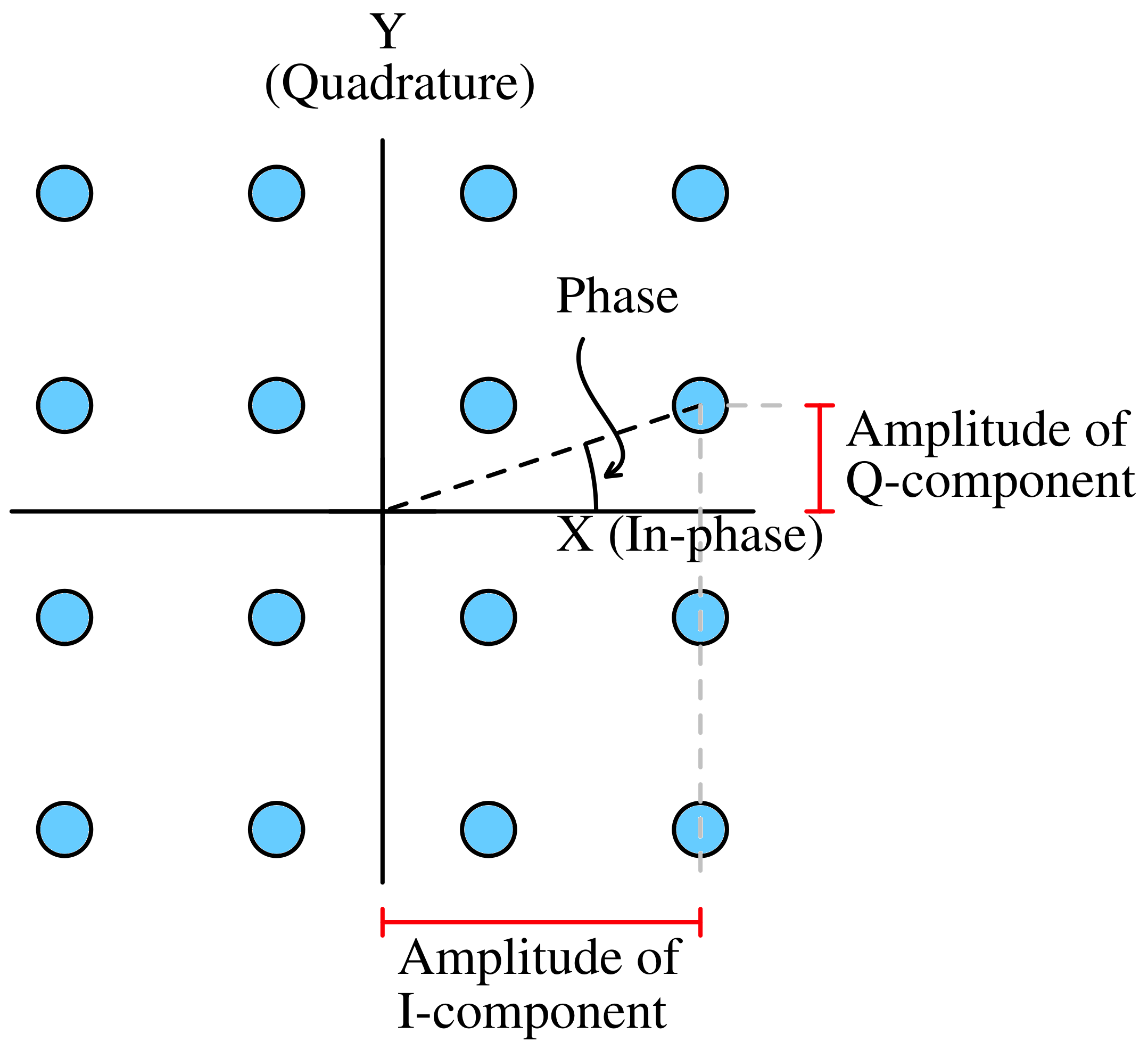
The In-phase (I) component is represented by the horizontal (x-axis). The Quadrature (Q) component is represented by the vertical (y-axis).
Orthogonal, orthonormal and basis functions
Basis functions are fundamental, orthogonal (ideally) signal shapes whose scaled combinations form a symbol in a constellation diagram. In-phase (i.e., sin(ωt)) and quadrature phase (i.e., cos(ωt)) are the basis functions in QPSK and QAM.
Orthogonal vectors are perpendicular to each other (their dot product is zero), while orthonormal vectors are orthogonal and also have a unit length (a magnitude of 1). The key difference is the requirement for unit length: all orthonormal sets are orthogonal, but not all orthogonal sets are orthonormal because their vectors might not have a length of 1.
Constellation diagram vs Vector diagram
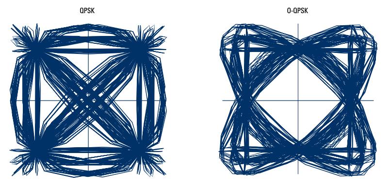
Constellation diagrams show decision points whereas Vector diagrams show the path the signal takes between decision points. Vector diagrams are drawn over constellation diagrams.
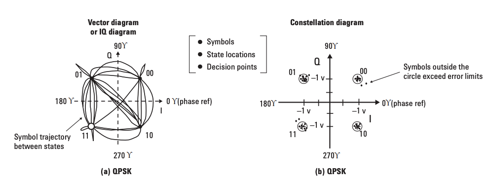
Vector diagram can differentiate between different modulation schemes e.g., QPSK and Offset-PSK.
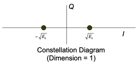
BPSK constellation
In binary phase-shift keying (BPSK) each symbol can only represent a 0 or a 1 because it has just two constellation points, therefore transmitting just one bit per symbol. The symbols are mathematically represented by s1 and s2 :
$$s_1(t)=\sqrt{\cfrac{2E_b}{T_b}}\cos(2\pi{}f_ct)\hspace{1cm}0\leq{}t\leq{}T_b$$
$$s_2(t)=-\sqrt{\cfrac{2E_b}{T_b}}\cos(2\pi{}f_ct)\hspace{1cm}0\leq{}t\leq{}T_b$$
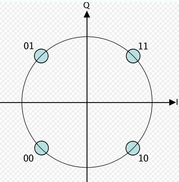
QPSK constellation
Quadrature phase-shift keying (QPSK), which has four constellation points, can represent 00, 01, 10, or 11, and can therefore transmit 2 bits per symbol.
QAM constellation
Some examples of QAM constellations are shown below :
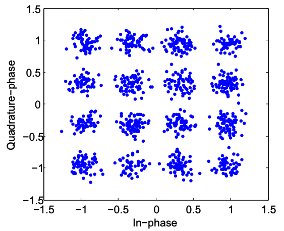
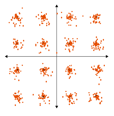
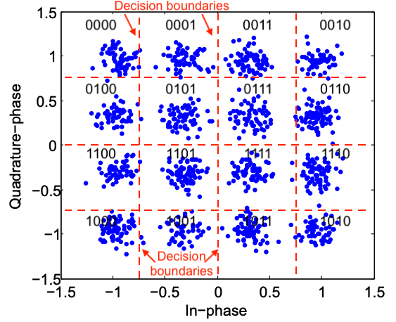
16-QAM modulation
The 16 blue dots represent the ideal magnitude and phase for each of the 16 symbols used in 16-QAM. The orange dots represent the measured signal’s magnitude and phase for each of the 16 symbols. Using constellation diagrams in this context, it is easy to visualize when a signal is performing well and when it is not. When a digital communication system is functioning as it should, the orange dots should be tightly clustered near each blue dots. When there is excess noise, distortion, spurious signals, or other problematic contributions degrading a signal’s integrity, magnitude and phase errors occur, causing the orange dots to deviate outside the blue dots defining the ideal signal locations.
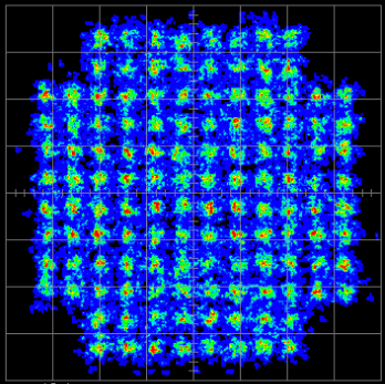
128-QAM constellation
A 128-QAM (Quadrature Amplitude Modulation) constellation is a digital signal representation consisting of 128 unique points, where each point (symbol) represents a specific combination of amplitude and phase. In this modulation scheme, each symbol conveys 7 bits of information (27=128).
Performance & Analysis Metrics
The properties of a modulation scheme can be inferred from its constellation diagram. As the number of signal points per dimension increases, the constellation becomes more dense, leading to higher spectral efficiency and hence a reduction in the bandwidth required for a given data rate. However, the probability of bit error is inversely proportional to the distance between the closest constellation points. As this distance decreases in denser constellations, the system becomes more sensitive to noise and impairments, resulting in a higher error rate.
Symbol decision boundary
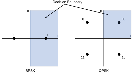
Symbol decision boundaries are lines (or surfaces in higher dimensions) that divide the space into regions, each assigned to a specific transmitted symbol.
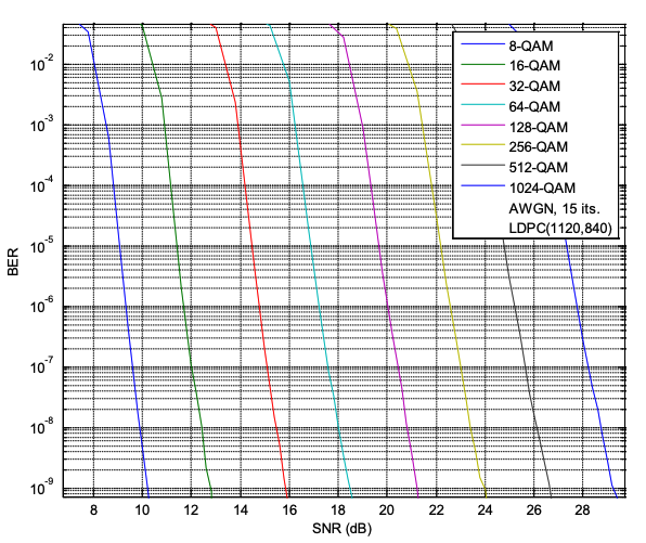
From the above graph, it can be observed that achieving the same bit error rate (BER) requires a higher signal-to-noise ratio (SNR) for higher-order QAM schemes.
This is because, as the modulation order increases, the constellation becomes denser and the spacing between symbols decreases for the same average signal power. Since the noise level remains unchanged, symbols are more likely to cross the decision boundaries, resulting in a higher probability of error. Therefore, to maintain the same BER, the signal power must be increased, leading to a higher required SNR.
Error vector magnitude (EVM)
EVM is the scalar distance between the end points of the measured and ideal phasors, and is a measure of how well a digital communications system is performing. To obtain the EVM, a constellation based on a large number of detected samples is constructed and a vector is drawn between each measured point and its ideal position.
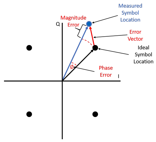
EVM is typically expressed as a percentage (%) or in decibels (dB). It is the ratio of the Root Mean Square (RMS) power of the error vector to the RMS power of the ideal reference.
$$\text{EVM (%)}=\sqrt{\cfrac{|V_{error}|}{|V_{ideal}|}}\times{}100\%$$
EVM characterizes the accuracy of a received waveform at the symbol sampling instants and is therefore directly related to the bit error rate (BER) in digital radio systems. EVM captures the combined effects of multiple impairments, including power amplifier nonlinearities, amplitude and phase imbalances between the I and Q signal paths, in-band amplitude ripple (for example due to filters), noise, non-ideal mixing, imperfect carrier recovery, and DAC inaccuracies.
Modulation Error Ratio (MER)
A similar measure of signal quality is the modulation error ratio (MER), a measure of the average signal power to the average error power. In decibels it is defined as:
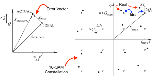
$$\text{MER}|_{dB}=10\log_{10}\cfrac{(1/N)\sum{}_{i=1}^{N}(I_i^2+Q_i^2)}{(1/N)\sum{}_{i=1}^{N}(\Delta{}I_i^2+\Delta{}Q_i^2)}=10\log_{10}\cfrac{\sum{}_{i=1}^{N}(I_i^2+Q_i^2)}{\sum{}_{i=1}^{N}(\Delta{}I_i^2+\Delta{}Q_i^2)}$$
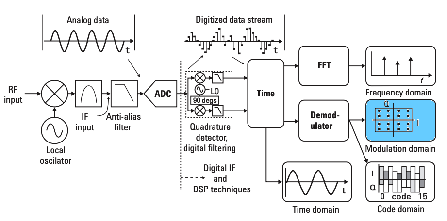
Measurement & Visualization
To measure a constellation diagram, the digital modulated signal is first captured using a vector signal analyzer (VSA) or a high-bandwidth oscilloscope. The instrument then demodulates the received signal into its in-phase (I) and quadrature (Q) components, which form the X- and Y-axes of the constellation diagram, respectively. Each sampled symbol is plotted as a point in the I–Q (complex) plane, resulting in a cloud of points corresponding to the modulation states.
Tightly clustered points indicate an ideal, high-quality signal with minimal noise or interference
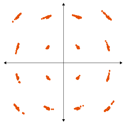
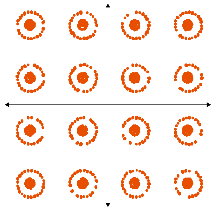
Phase error
Phase noise forms arcs of noise at the symbol points. Caused by high phase noise in local oscillator or carrier.
Amplifier compression
Points pulled inward toward the origin imply amplifier compression and nonlinearity.
Low SNR
Widely scattered points indicate high noise, interference, or a poor signal-to-noise ratio (SNR).
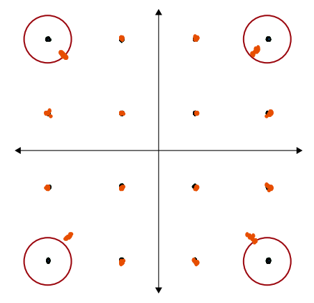
In-band spurious
A spurious continuous-wave (CW) signal within the channel bandwidth causes the constellation points to form a characteristic “donut” or ring-shaped pattern. This occurs because the unwanted CW tone adds a rotating phasor to the desired modulated signal, producing a constant-magnitude but time-varying phase error. Typical sources of such spurs include switching power supply clocks or other oscillators in the device under test (DUT) that leak into the I/Q modulator or local oscillator path, thereby corrupting the constellation.
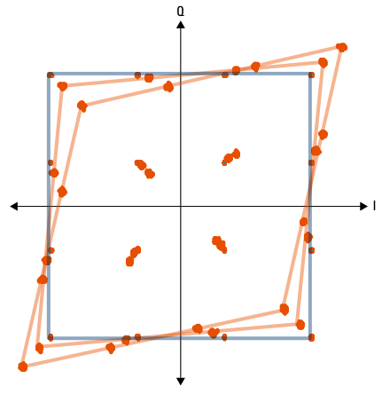
IQ Quadrature error
Quadrature error results when the angle between I and Q is not 90°. This problem distorts the constellation from a square to a parallelogram.
Carrier frequency error
Carrier frequency error is the difference between the actual output center frequency and the intended (nominal) carrier frequency. It arises from inaccuracies or drift in the device under test (DUT)’s frequency reference, such as crystal tolerance, aging, temperature variation, or reference clock instability. Frequency error is not visible in the constellation however VSA manufacturers provide result summary to indicate carrier frequency error.
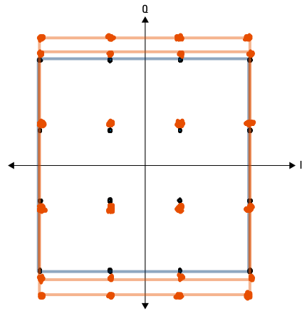
IQ Imbalance
Ideally, the I and Q channels should have equal gain, and this equal gain gives most QAM constellations their characteristic “square shape”. I/Q gain imbalance occurs when there is a difference between the gain of the I component and the Q component. I/Q gain imbalance causes the constellation to be distorted to a rectangule than a square.
There are two mathematical models of IQ imbalance 1 :
- The Double-branch IQ imbalance model (DBIQM)
- The Single-branch IQ imbalance model (SBIQM)
IQ Imbalance models
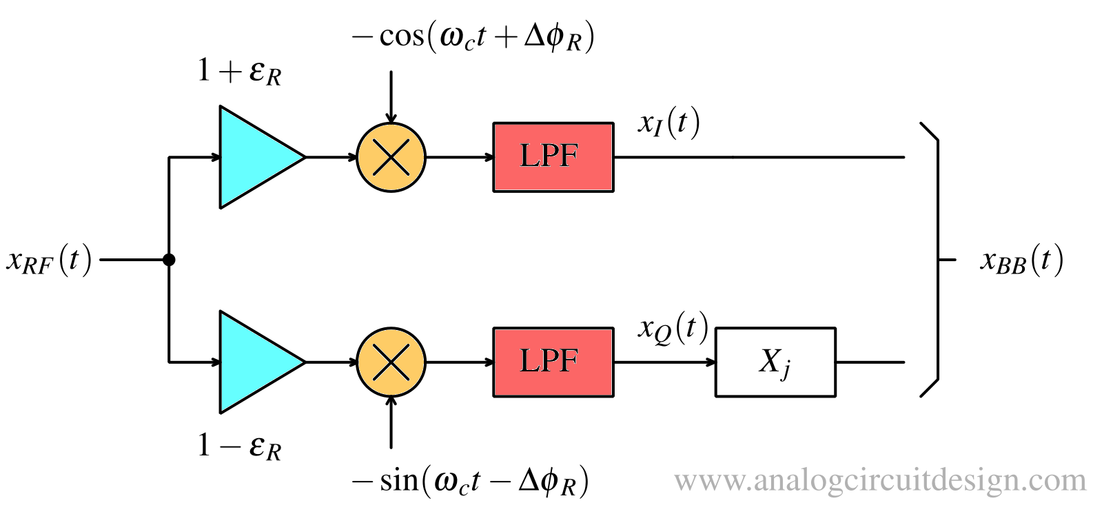
The Double-branch IQ imbalance model
In this model the mismatch between the I and Q branches is represented by errors in both the I and Q branches (worst cases). In the I branch, the amplitude and phase mismatch are characterized by (1+εR) and +Δφ respectively. In the Q branch, the amplitude and phase imbalance are characterized by (1-εR) and -Δφ. In case of not having any IQ imbalance, then the values of both εR, and Δφ are zero. The IQ-imbalanced signal using the DBIQM can be modelled as follows:
$$\begin{bmatrix}x_{FI}(t) \\ x_{FQ}(t)\end{bmatrix}=\begin{bmatrix}(1+\epsilon{}_R)\cos{(\Delta{}\phi{}_R)} & (1+\epsilon{}_R)\sin{(\Delta{}\phi{}_R)} \\ (1-\epsilon{}_R)\sin{(\Delta{}\phi{}_R)} & (1-\epsilon{}_R)\cos{(\Delta{}\phi{}_R)}\end{bmatrix}\begin{bmatrix}x_{I}(t) \\ x_{Q}(t)\end{bmatrix}$$
The signal to distortion ratio (SDR) amount in dB due to IQ imbalance using DBIQM can be found by the following formula. $$\text{SDR}=10\log_{10}\left(\cfrac{1+\epsilon{}_R^2+\epsilon{}_R^2\tan^2(\Delta{}\phi{}_R)}{\epsilon{}_R^2+\tan^2(\Delta{}\phi{}_R)}\right)$$
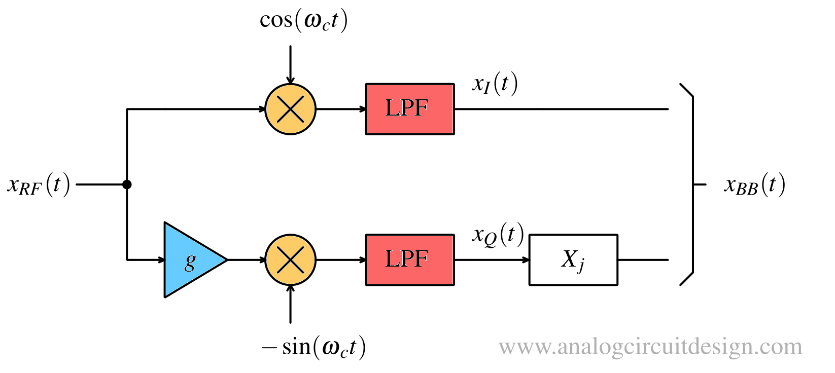
The Single-branch IQ imbalance model
In this model the mismatch between the I and the Q branches exists only in the Q branch, and there is no error in the I branch. The amplitude gain in the Q branch is characterized by g and the phase mismatch is characterized by φ, Therefore, for this model, 1-g represents the amount of error in the amplitude. The IQ-imbalanced signal using the SBIQM can be modelled as follows:
$$\begin{bmatrix}x_{FI}(t) \\ x_{FQ}(t)\end{bmatrix}=\begin{bmatrix}1 & 0 \\ -g\sin{(\phi)} & +g\cos{(\phi)}\end{bmatrix}\begin{bmatrix}x_{I}(t) \\ x_{Q}(t)\end{bmatrix}$$