Modulation
Modulation is the process of "mounting" a low-frequency information signal (like your voice) onto a high-frequency carrier wave by changing its properties like amplitude, phase, or frequency. The primary reason of modulation of high frequency carrier wave is to reduce the size of antenna.
Intuition
Imagine trying to throw a piece of paper across a room; it won't go far. But if you wrap that paper around a stone and throw it, the paper reaches the destination. Here, the paper is your data, the stone is the carrier wave, and wrapping them together is modulation.
Related terminologies
Some important and common terminologies related to modulation are listed below:
Spectral efficiency
Spectral efficiency measures how efficiently a communication channel transmits data. It is defined as the net bit rate (useful information rate excluding error-correction overhead), or throughput, divided by the occupied RF bandwidth. Spectral efficiency is expressed in bits per second per hertz (bits/second-Hz).
$$\text{Spectral Efficiency}=\cfrac{\text{Capacity in bits/sec}}{\text{Bandwidth in kHz}}$$
Symbol rate vs Bit rate
$$\text{Bit Rate}=\cfrac{\text{Symbol Rate}}{\text{Bits per symbol}}$$
bits per symbol = log2(M) for an M-ary modulation where each symbol maps to one of M distinct states (e.g., QPSK where M=4 has 2 bits/symbol; 16-QAM where M=16 has 4 bits/symbol)
Modulation depth or modulation index
Modulation Index and Modulation Depth are used interchangeably. Modulation Depth is simply modulation index expressed in percentage.
In AM, modulation index (m) is the ratio of the peak amplitude of the modulating signal to the peak amplitude of the carrier signal. A modulation index m = 0 indicates no modulation, corresponding to an unmodulated carrier. A modulation index m = 1 represents full modulation, in which the carrier amplitude varies from zero to its maximum value.
In FM, the modulation index (β) is defined as the maximum frequency deviation (Δf) divided by the frequency of the modulating signal (fm).
Error vector magnitude (EVM)
Error Vector Magnitude (EVM) measures the difference between the ideal symbol position in a constellation diagram and the actual received (or transmitted) symbol. More about Error Vector Magnitude : EVM
Mixer
An RF Mixer is a three-port circuit element that translates a signal from one frequency to another. Mixers work through the multiplication of two signals in the time domain. It is symbolized by a cross sign in circuit diagrams.
Analog Modulation
In analog (or continuous-wave) modulation, an analog carrier signal is modulated using an analog baseband (message) signal. The message signal varies one of the carrier’s parameters like amplitude, frequency, or phase. Accordingly, analog modulation is classified into amplitude modulation (AM), frequency modulation (FM), and phase modulation (PM). Amplitude modulation is referred to as linear modulation, while frequency and phase modulation together are known as angle modulation.
Amplitude Modulation
It is the process in which the amplitude of a sinusoidal carrier varies in accordance with the instantaneous value of the message (modulating) signal.
$$x_{AM}(t)=[A_c+x_{BB}(t)]\cos(\omega{}_ct)$$
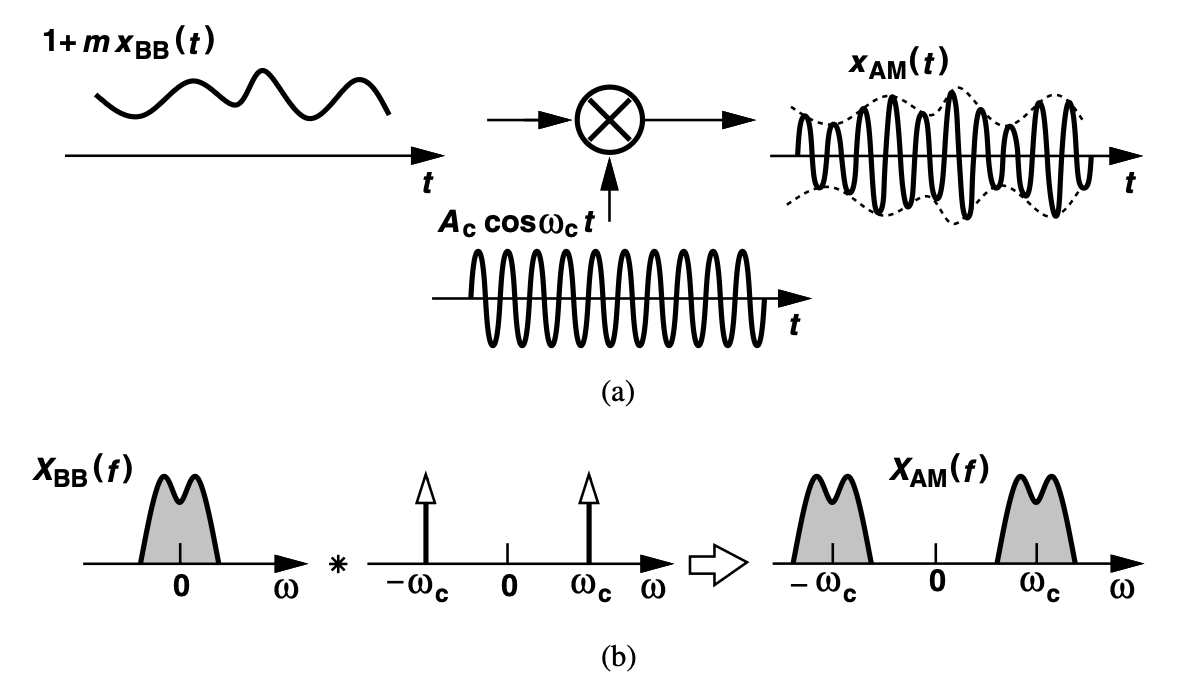
Multiplying by cos(ωct) in the time domain shifts the spectrum of xBB(t) to be centered at ωc, a process known as upconversion. As a result, the bandwidth of the AM signal xAM(t) becomes twice that of the baseband signal. Since xBB(t) is a real signal with a spectrum symmetric about zero frequency, the spectrum of xAM(t) is also symmetric around ωc. This symmetry is not present in all modulation schemes and decides transceiver architecture design.
The modulation index in AM can be represented as :
$$m=\cfrac{|x_{BB}|_{max}}{A_c}$$
Phase modulation
In Phase modulation, phase angle of sinusoidal carrier wave (argument of cosine/sine function) changes in accordance with the instantaneous value of a message or modulating signal (xBB(t)). The amplitude is kept constant as shown below :
$$x_{PM}(t)=A_c\cos(\omega{}_ct+m\times{}x_{BB}(t))$$
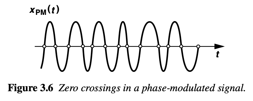
To understand phase modulation intuitively, first observe that when xBB(t)=0, the zero-crossing points of the carrier occur at uniformly spaced instants equal to integer multiples of the period Tp = 1/2πωc. When xBB(t) varies with time, however, the zero crossings shift according to the modulation, while the carrier amplitude remains constant.
Frequency Modulation
It is the process in which the frequency of a sinusoidal carrier wave varies in accordance with the instantaneous value of the message (modulating) signal. Mathematically it is expressed as :
$$x_{FM}(t)=A_c\cos(\omega{}_ct+m\int_{-\infty}^{t}x_{BB}(t)dt)$$
The instantaneous frequency is ωc+mxBB(t). The frequency is directly proportional to the base-band (message signal) so it is called frequency modulation.
Narrowband FM approximation
If xBB(t)=Acos(ωmt), then :
$$x_{FM}(t)=A_c\cos\left(\omega{}_ct+\cfrac{mA_m}{\omega{}_m}\sin(\omega{}_mt)\right)$$
A special case of FM that proves useful in the analysis of RF circuits and systems arises if mAm/ωm < 1 rad. The signal can be approximated as :
$$x_{FM}(t)=A_c\cos(\omega{}_ct)-A_mA_c\cfrac{m}{\omega{}_m}\sin(\omega{}_mt)\sin(\omega{}_ct)$$
$$x_{FM}(t)=A_c\cos(\omega{}_ct)-\cfrac{mA_mA_c}{2\omega{}_m}\cos(\omega{}_c-\omega{}_m)t+\cfrac{mA_mA_c}{2\omega{}_m}\cos(\omega{}_c+\omega{}_m)t$$
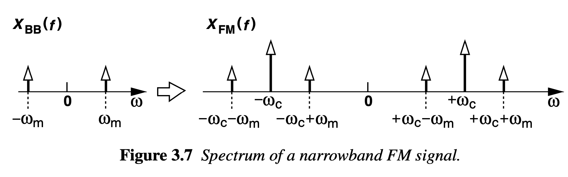
Note that the coefficients of sidebands in narrowband FM are opposite.
Digital Modulation
In digital modulation, an analog carrier is modulated using a digital baseband (message) signal. For instance, the voice captured by a mobile phone microphone is first digitized by an ADC and then used to modulate the carrier. In contrast, analog modulation directly uses the microphone signal to modulate the carrier. Representing information in digital form provides many advantages compared to analog communication.
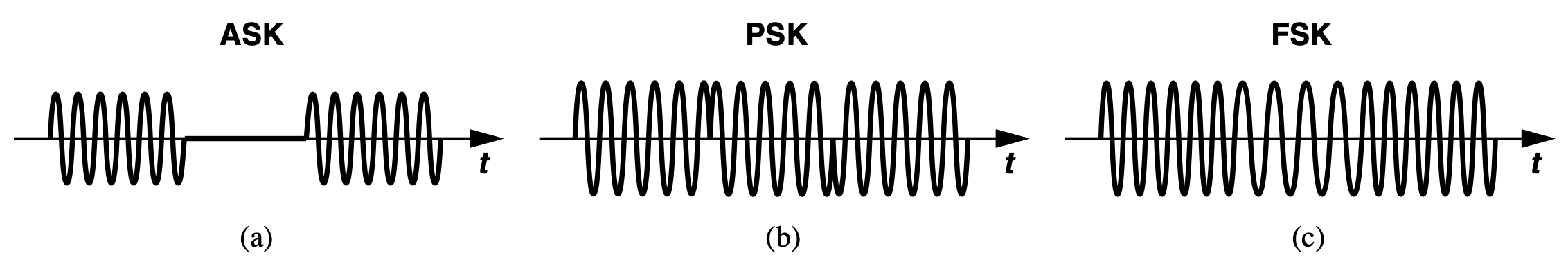
ASK
In ASK, the baseband data switches between +1 (logic "high") and 0 (logic "low"), multiplying this waveform with the carrier produces a ASK signal. It is also known as “on-off keying” (OOK). It is the digital counterpart of AM.
PSK
In PSK, the baseband data switches between two or more distinct frequencies. If the signal switches between only +1 (logic "high") and −1 (logic "low") it is called Binary PSK. It results in a zero-mean signal, multiplying this waveform with the carrier produces a PSK signal. This is because each data transition reverses the sign of the carrier, causing a 180° phase shift. It is the digital counterpart of PM.
FSK
In Frequency Shift Keying (FSK) the carrier frequency is shifted between predefined discrete frequencies according to the binary input data. A logical “1” and “0” are transmitted by changing the carrier to one of two distinct frequencies during each bit interval. It is the digital counterpart of FM. FSK class of modulation schemes does not require linear power amplifiers because it is a “constant-envelope modulation”, thus exhibiting high power efficiency. The frequency modulation is done using a VCO.
ISI and Pulse shaping basics
Inter-Symbol Interference (ISI) is the phenomena where distortion due to band-limitation of the channel causes transmitted symbol's energy spread into adjacent symbols, causing them to become unreadable, leading to data errors.
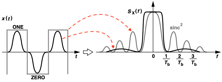
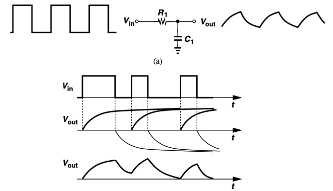
Pulse shaping is a technique used to reduce the bandwidth required by a modulated signal by designing shape of the baseband pulse (like raised cosine) to inherently occupy a smaller bandwidth. Smoother transitions between ONEs and ZEROs in the baseband signal can tighten the spectrum. Rectangular pulse because of its sharp transitions between zeros and ones require an unnecessarily wide bandwidth.
Signal Constellations
Quadrature Modulation
Binary PSK signals that use square baseband pulses of width Tb seconds occupy a total bandwidth much wider than 2/Tb hertz after upconversion to RF. Applying baseband pulse shaping can reduce this bandwidth to approximately 2/Tb. To achieve even greater bandwidth efficiency, quadrature modulation, specifically quadrature PSK (QPSK), can be used.
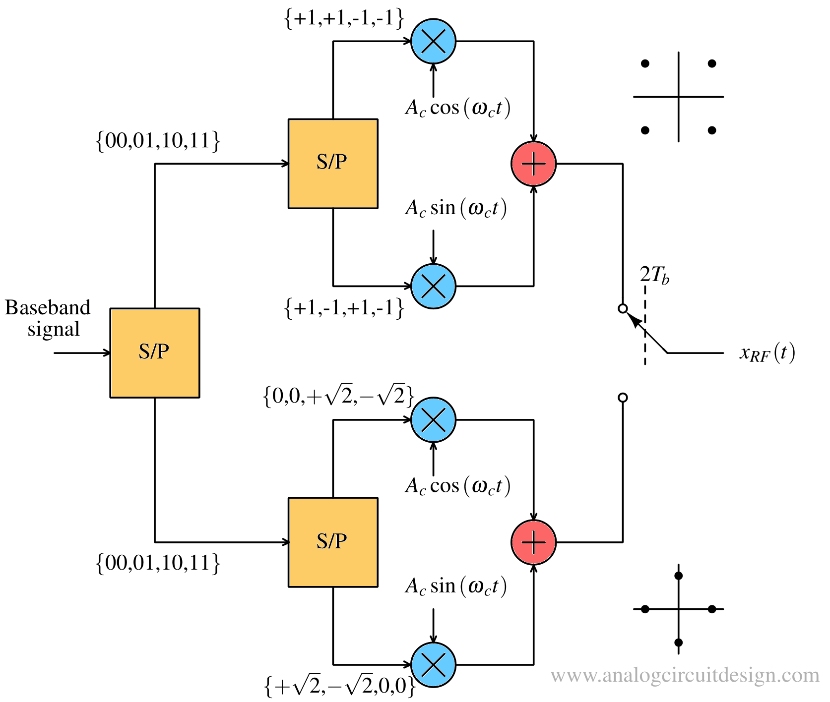
QPSK
In QPSK, the binary serial data stream is divided into two parallel bits, and each bit is mapped onto the quadrature phases of the carrier, i.e., cos(ωct) and sin(ωct):
$$x_c(t)=b_{2m}A_c\cos{\omega{}_ct}-b_{2m+1}A_c\sin{\omega{}_ct}$$
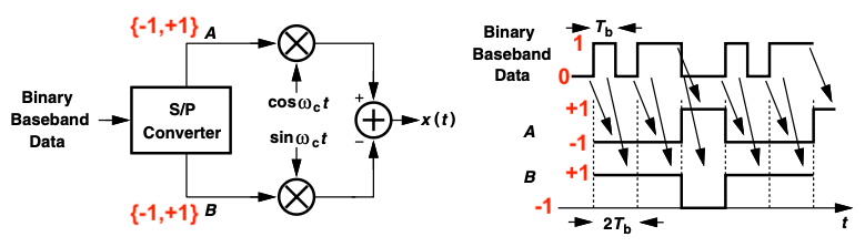
QPSK modulation halves the occupied bandwidth. This is simply because the demultiplexer “stretches” each bit duration by a factor of two before giving it to each arm. The “symbol rate” of QPSK is half of its bit rate.
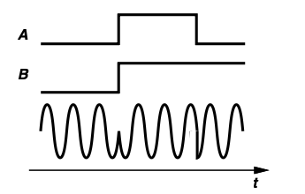
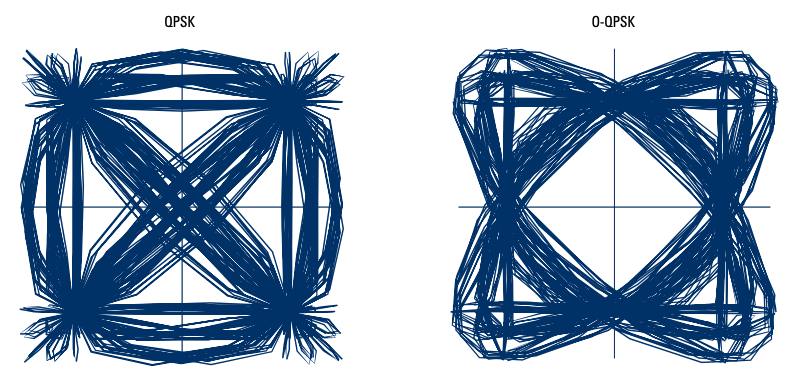
An important drawback of QPSK stems from the large phase changes at the end of each symbol as shown above. To limit the transmission bandwidth, pulse shaping is required. However, pulse-shaping leads to variable envelope as shown below :
A variable-envelope signal requires a linear power amplifier, which is inevitably less efficient than a nonlinear power amplifier.
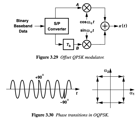
Offset QPSK (OQPSK)
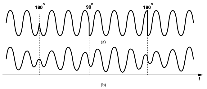
A variant of QPSK that remedies the above drawback is “offset QPSK” (OQPSK). The parallel data streams (A and B) are offset in time by half the symbol period (Tb) after the demultiplexer, thereby avoiding simultaneous transitions in waveforms at nodes A and B. Simulatenous transition leads to complete 180° phase movement, leading to sharp transients. In OQPSK, the phase step therefore does not exceed ±90°.
Main drawback of OQPSK is that it loses ability of differential encoding which is important for noise immunity.
π/4 QPSK
A variant of QPSK that can be differentially encoded is “π/4-QPSK”. It allows smoother transition. The signal set consists of two QPSK schemes, one rotated 45° with respect to the other:
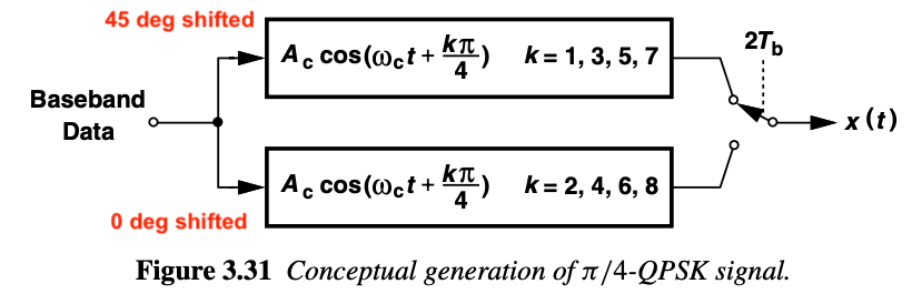
There are two QPSK modulators operating in parallel. One it generating 45°, 135°, 225°, 315° phase shifted signals. Other is generating 0°, 90°, 180°, 270° phase shifted signals. Through baseband pulse shaping, QPSK and its variants achieve high spectral efficiency, but they suffer from poor power efficiency because envelope variations require the use of linear power amplifiers.
GMSK Modulation
A widely used pulse-shaping technique for frequency modulation employs a Gaussian filter, whose impulse response is a Gaussian pulse. When rectangular pulses are applied directly to a VCO input, the resulting frequency transitions are abrupt requiring larger bandwidth. By smoothing these pulses before the VCO, the frequency changes become more gradual, producing a narrower output spectrum.
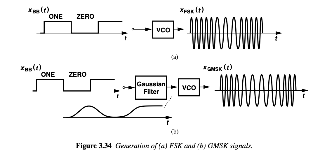
The GMSK waveform can be expressed as :
$$x_{GMSK}(t)=A_c\cos\left[\omega{}_ct+m\int{}\{x_{BB}(t)*h(t)\}dt\right]$$
where h(t) denotes the impulse response of the gaussian filter. "m" is the modulation index and it is a dimensionless quantity here. It has a value of 0.5. Due to its constant-envelope property, GMSK enables power amplifiers to be optimized for high efficiency with minimal concern for linearity.
GFSK Modulation
A slightly different version of GMSK, called Gaussian frequency shift keying (GFSK), is employed in Bluetooth. The GFSK waveform is similar to GMSK waveform given by following equation but with modulation index "m" = 0.3:
$$x_{GFSK}(t)=A_c\cos\left[\omega{}_ct+m\int{}\{x_{BB}(t)*h(t)\}dt\right]$$
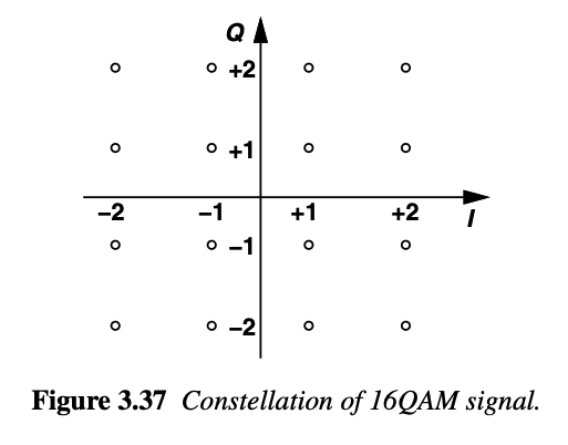
Quadrature Amplitude Modulation (QAM)
In Quadrature amplitude modulation (QAM), both amplitude and phase can vary. Simplest QAM is QPSK where the amplitude can be just ±1.
In higher QAM scheme, the amplitudes can be ±1 and ±2. The final carrier waveform can be expressed as :
$$y(t)=A_1\sin(\omega{}_ct)+A_2\cos(\omega{}_ct)$$
A1 and A2 can assume values from +1,-1,+2,-2 creating 16 distinct waveforms. Therefore this QAM is called 16-QAM. 16-QAM reduces the bandwidth requirement by 4 times against BPSK. For a given transmit power, the constellation points are closer together than in a simple QPSK, making detection more susceptible to noise. This increased noise sensitivity is the trade-off for improved bandwidth efficiency.
QAM can further reduce the required bandwidth compared to basic quadrature modulation techniques (QPSK, offset-QPSK etc).
QAM is the most adopted modulation scheme. It has been central to increasing data rates and system capacity by packing more information onto a carrier and utilizing fixed channel bandwidths more efficiently, approaching Shannon’s limit. As a result, QAM is widely used in cellular networks, WiFi access (such as 802.11), and satellite communications etc.
Orthogonal Frequency Division Multiplexing
Multipath propagation in wireless channels causes delay spread, which can result in severe intersymbol interference (ISI). Orthogonal frequency-division multiplexing (OFDM) is an effective technique for mitigating the effects of this delay spread.
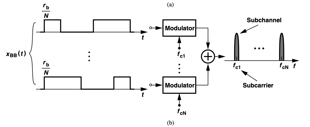
In OFDM, the baseband data stream is first demultiplexed by a factor of N, creating N parallel streams, each with a symbol rate of rb/N. These streams are then modulated onto N different carrier frequencies, from fc1 to fcN, forming a multicarrier spectrum. Although the overall bandwidth and data rate remain the same as those of a single-carrier system, the multicarrier signal is less sensitive to multipath effects because each carrier conveys a lower-rate data stream and can therefore tolerate a larger delay spread.