Phase noise
In RF-wireless and broadband wired communication systems, phase noise and Jitter are critical parameters associated with clock generators (oscillators). Phase noise (or PN) is the short-term variations in phase or frequency stability, with "short term" referring to time intervals comparable to time period of the clock (or oscillator). It is random or unintentional phase modulation. These phase modulations in the clock edges (or zero-crossings) leading to localized variation of time periods called Jitter.

Phase noise term is more relevant in wireless technologies. Jitter term is more relevant in wired technologies (e.g., Ethernet, optical communication), intra-chip and inter-chip communication.
The main factors causing phase noise and jitter include transistor noise, resistor noise, power supply variations, loading conditions, device noise, and interference coupled from nearby circuits.
Relationship between Phase-noise and Jitter
To observe the difference between jitter and phase noise, consider the sine wave signal:
$$X(t)=\sin\left(2\pi{}f_0t+\phi{}(t)\right)$$
Where fo is the nominal frequency, and \(\phi(t)\) is the phase noise or variations. To see the relationship to jitter (Δt(t), time difference as a function of t) the preceding equation is rewritten as:
$$X(t)=\sin\left(2\pi{}f_0\left(t+\cfrac{\phi{}(t)}{2\pi{}f_0}\right)\right)$$
Now the time-jitter (Δt(t)) and phase noise (φ(t)) are related by following mathematical relation:
$$\Delta{}t(t)=\cfrac{\phi{}(t)}{2\pi{}f_0}$$
Phase noise, as used in RF applications, is often represented in frequency domain rather than the time domain. The PSD of phase noise can be represented as Sφ(f). The units of phase noise PSD is rad2/Hz. The above relation can be used to convert phase noise into jitter by squaring both sides:
$$S_{\Delta{}t}(f)=\cfrac{1}{(2\pi{}f_0)^2}S_{\phi{}}(f)$$
The units of SΔt(f) are sec2/Hz and represents the PSD of jitter. We can get the RMS form of jitter (JRMS) from the same relation:
$$J_{RMS}=\sqrt{\int_{f_L}^{f_H}S_{\Delta{}t}(f)df}=\cfrac{1}{2\pi{}f_0}\sqrt{\int_{f_L}^{f_H}S_{\phi{}}(f)df}$$
The integral inside the square root represents the area under phase noise PSD curve. A good document explaining it further - Converting Oscillator Phase noise to Time Jitter.
Problems due to Phase noise
Phase noise is problematic in RF signal chains. It can cause following problems:
Reciprocal mixing
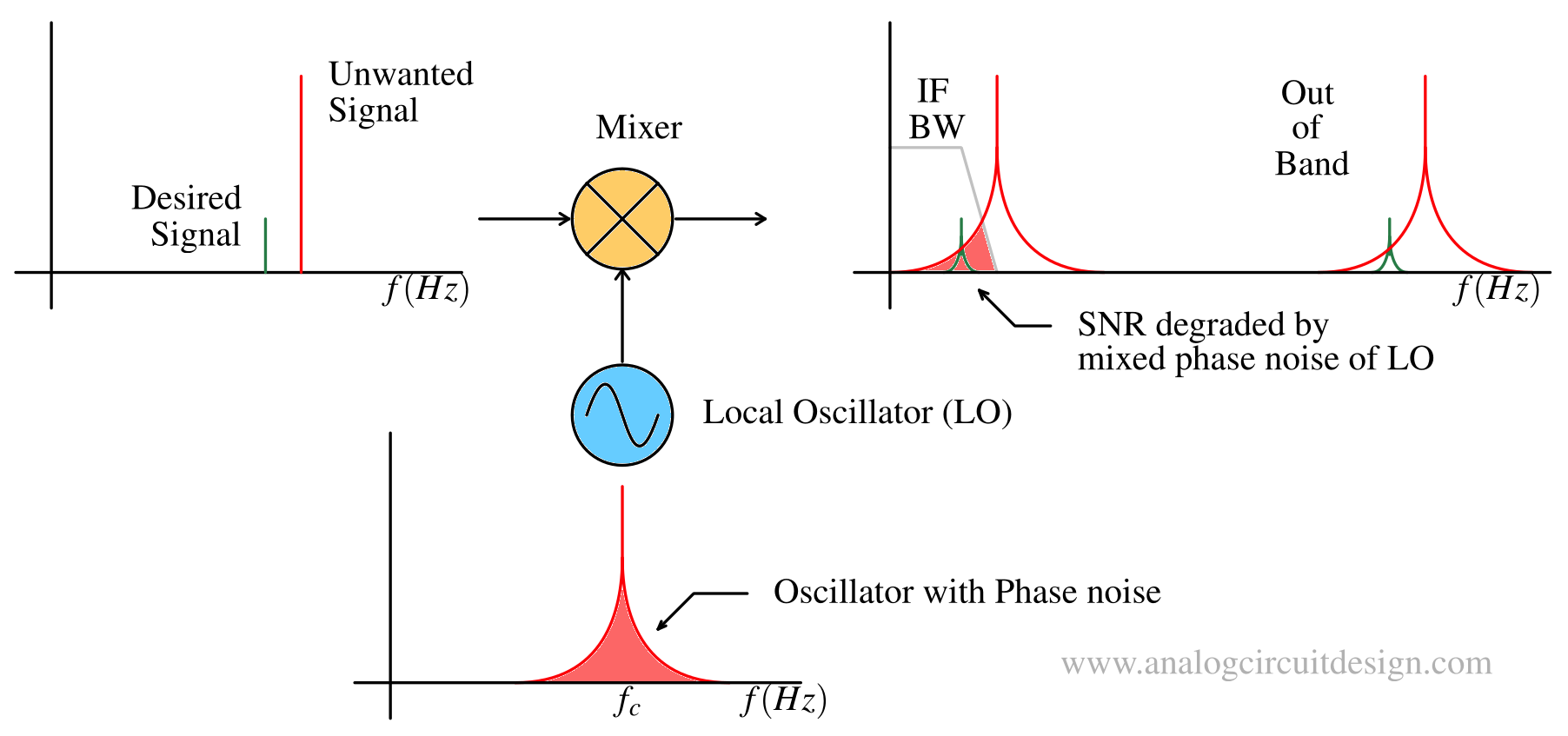
At the receiver, a large interferer can degrade the SNR of the wanted signal due to “reciprocal mixing” caused by the LO phase noise. The LO phase noise mixes with both desired and adjancent channel carrier. The spread of phase noise of adjancent channel leaks into the IF filter bandwidth which cannot be attenuated. Thus, noise level increases as shown above.
Spectral regrowth
Spectral regrowth is the unwanted generation of new frequency components (intermodulation products) around a main carrier signal, caused by nonlinearities and phase noise of the components in the signal chain.
More details about Spectral Regrowth - Spectral Regrowth
Increased BER
Most modern wireless technologies use modulation schemes that are often representation using constellation diagrams, and phase noise causes a rotation of this constellation, with higher phase noise causing greater rotation and a higher bit error rate.
Phase noise plot or spectrum
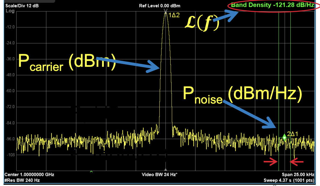
Phase noise measured using spectrum analyzer. Source : Keysight Technologies.
As shown in the above figure, the phase noise appears as noisy continuum of sidebands (or skirt) around the carrier frequency. Both the sidebands of are symmetrical therefore for convenience, only the Single Side Band (SSB) is used for analysis.
Mathematically the phase noise, φn(t) for a carrier signal Acos(ω0t) can be modelled as :
$$y(t)=A\cos\left(\omega_0t+\phi{}_n(t)\right)$$ $$\simeq{}A\cos\left(\omega{}_ct\right)\cos\left(\phi{}_n(t)\right)-A\sin\left(\omega{}_ct\right)\sin\left(\phi{}_n(t)\right)$$ The noise is relatively small with respect to ω0t, So we can make a safe approximation as follows: $$\simeq{}A\cos\left(\omega{}_ct\right)-\underbrace{A\sin\left(\omega{}_ct\right)\phi{}_n(t)}_{\text{PN amplitude modulated}}$$
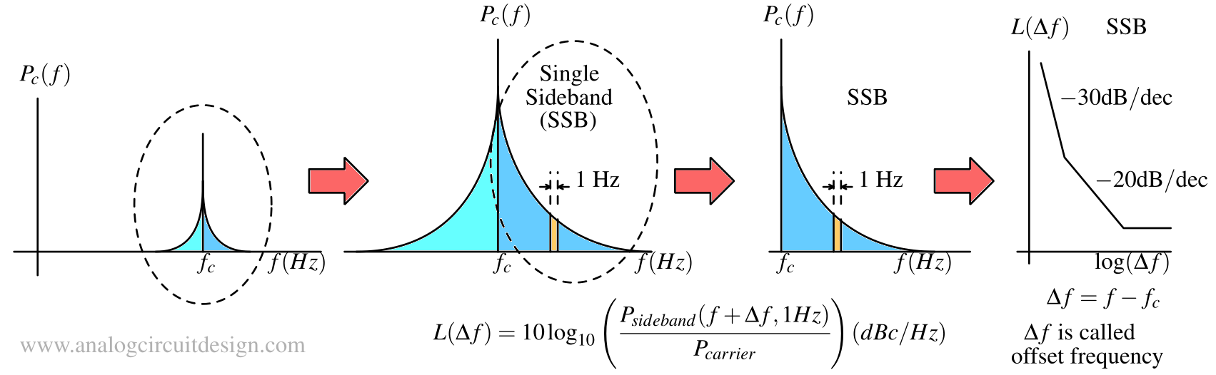
Three important elements of Phase noise measurements are :
- Offset frequency (Δf) from carrier frequency (fc) Since the phase noise falls at frequencies farther from carrier frequency, it must be specified at a certain “frequency offset,” i.e., a certain difference with respect to carrier frequency.
- Power spectral density relative to carrier power Carrier power and Phase noise power are in dBm. The relative power is represented as dBc.
- Power spectral density in 1Hz bandwidth At high carrier frequencies, it is difficult to measure the noise power in a 1-Hz bandwidth. The power could be represented for higher bandwidth, we have to convert the power for 1Hz bandwidth and measure the spectral density.
Problem
Suppose a spectrum analyzer measures a noise power of -65 dBm in a 1-kHz bandwidth at 1-MHz offset. How much is the phase noise at this offset if the average oscillator output power is -5 dBm? $$\text{PSD}\times{}1\,\text{kHz}=1\,\text{mW}\times{}10^{-65\,\text{dBm}/10}\, \text{W}$$ $$\implies{}\text{PSD}=3.16\times{}10^{-13}\,\text{W/Hz}$$ $$\implies{}\text{PSD} (\text{in dB})=-95\,\text{dBm/Hz}$$ Absoulte Phase noise Power (PPN,abs) for 1Hz bandwidth, $$\implies{}P_{PN,abs}=\text{PSD}\times{}1\,\text{Hz}=-95\,\text{dBm}$$ Phase noise if carrier output power is -5 dBm : is $$P_{PN}=P_{PN,abs} - P_{C}=-95-(-5)=-90\,\text{dBc/Hz}$$
Close-in phase noise
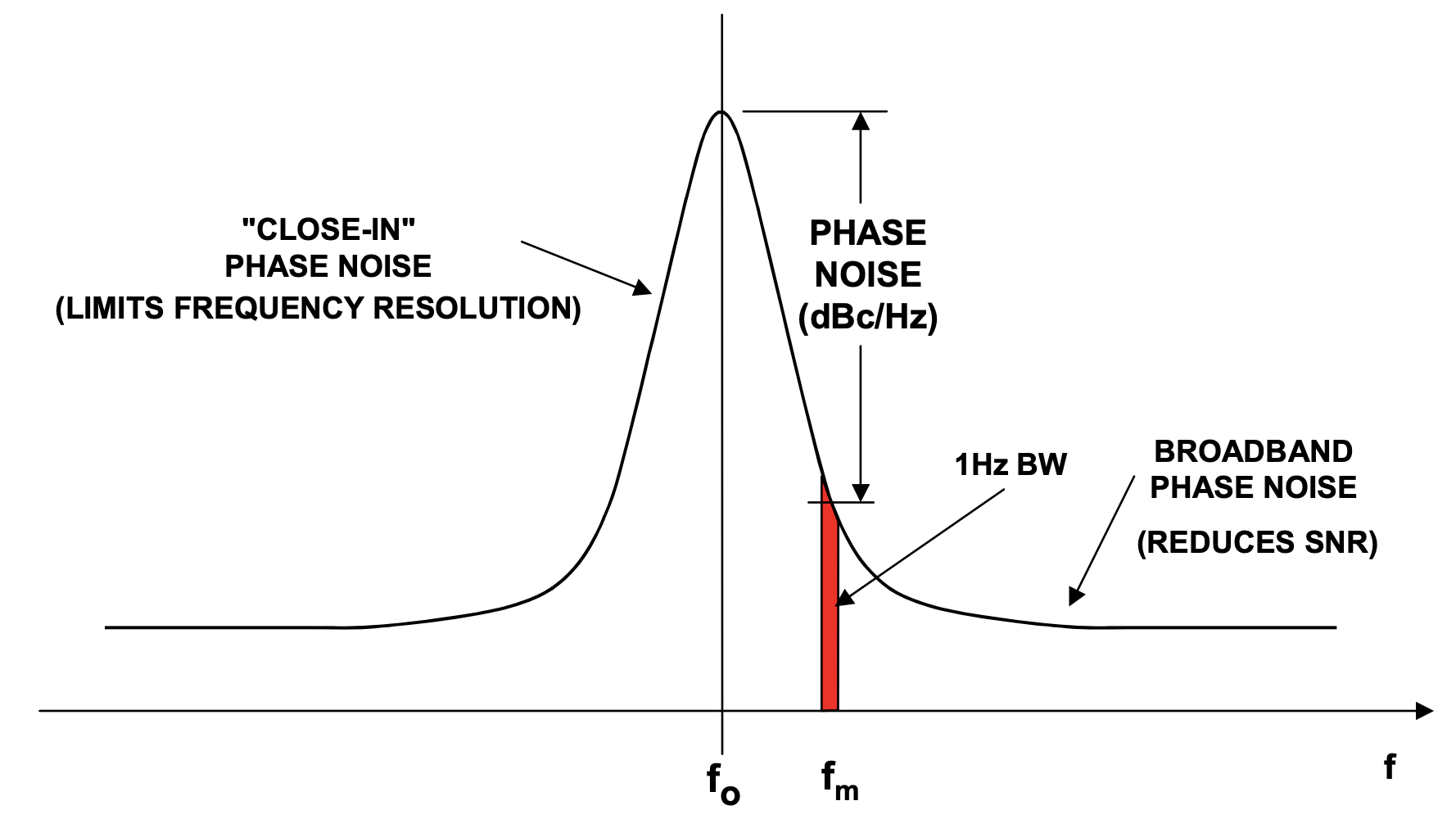
Close-in phase noise refers to unwanted random fluctuations (noise) in the phase of a signal, specifically measured at very small frequency offsets (e.g., < 1 kHz) from the main carrier frequency.
Far-from-carrier or Broadband phase noise
Far-from-carrier or Broadband phase noise is the constant noise floor observed at large frequency offsets from the central carrier frequency in a signal's spectrum. Typically the frequency offset is greater than 1MHz. It degrades the SNR because it folds back inside the intermediate frequency (IF) which is passband region.
Simple oscillator's phase noise model
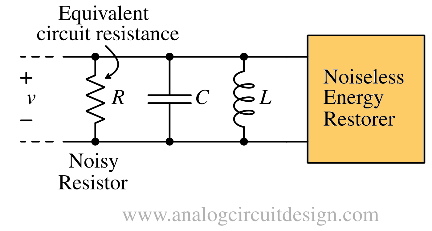
The spectral density of the mean-squared noise voltage is:
$$\cfrac{\bar{v_n}^2}{\Delta{}f}=\cfrac{\bar{i_n}^2}{\Delta{}f}\Big|\cfrac{1}{j\omega{}C}||(j\omega{}L)\Big|^2=\cfrac{\bar{i_n}^2}{\Delta{}f}\cfrac{j\omega{}L}{1-\omega{}^2LC}$$
For phase noise, we are interested in region close to resonance (ω0). The closeness is represented by Δω. Substituting ω=ω0+Δω and Q=ω0RC in the above equation:
$$\cfrac{\bar{v_n}^2}{\Delta{}f}=\cfrac{4kT}{R}\left(\cfrac{R\omega{}_o}{2Q\Delta{}\omega{}}\right)^2=4kTR\left(\cfrac{\omega{}_o}{2Q\Delta{}\omega{}}\right)^2$$
The output noise power spectral density is proportional to 1/Δf2 (-20dB/dec slope) due to bandpass filtering action on a flat (white) thermal noise. Additionally, increasing the tank quality factor Q lowers the noise density when all other parameters remain constant, highlighting the importance of using high-Q resonators2.
In the ideal LC oscillator model, the equipartition theorem states that, at equilibrium, the noise power is equally divided between amplitude and phase. As a result, the amplitude-limiting mechanism inherent in practical oscillators suppresses the amplitude noise, effectively eliminating half of the total noise. Therefore the remaining noise power can be represented by multiplication of 1/2 factor as shown below :
$$\cfrac{\bar{v_n}^2}{\Delta{}f}=2kTR\left(\cfrac{\omega{}_o}{2Q\Delta{}\omega{}}\right)^2$$
The noise power density equation above is normalized and then converted to a logarithmic scale by taking the logarithm of both sides. It is represented as L:
$$L\{\Delta{}\omega{}\}=10\log_{10}\left[\cfrac{2kT}{P_{carrier}}\left(\cfrac{\omega{}_o}{2Q\Delta{}\omega{}}\right)^2\right]$$
Where,
$$P_{carrier}=\cfrac{V_{carrier}^2}{R}$$
The unit of above equation is dBc/Hz.
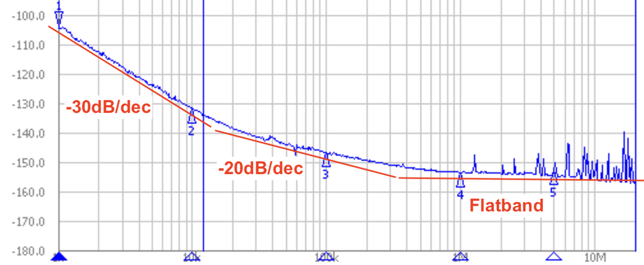
Leeson's model
The simple oscillator's phase noise model is only explaining the -20dB/dec slope. There are two more regions one having -30dB/dec and another is flat.
To explain this, Leeson introduced following equation:
$$L\{\Delta{}\omega{}\}=10\log_{10}\left[\cfrac{2kTF}{P_{carrier}}\left\{1+\left(\cfrac{\omega{}_o}{2Q\Delta{}\omega{}}\right)^2\right\}\left(1+\cfrac{\Delta{}\omega{}_{1/f^3}}{|\Delta{}\omega{}|}\right)\right]$$
F and Δω1/f3 are measurement based fitting constants. Δω1/f3 is expected to match the flicker noise corner ω1/f of the transistor however measurement shows it does not match.
The original Leeson's paper : A simple model of feedback oscillator noise spectrum
Lee-Hajimiri model
To explain F and Δω1/f3 further which can help us identify more parameters to optimize phase noise, Lee-Hajimiri proposed "A linear time-varying phase noise" model. Due to amplitude limiting nature of oscillators, they are non-linear. Linear Time-Invariant systems cannot perform frequency translations. They demonstrated that ideal LC oscillator's phase impulse response is time variant and introduced something called Impulse sensitivity function (ISF). The impulse sensitivity function is represented by Γ(ωoτ) in the phase impulse response hφ(t,τ):
$$h_{\phi{}}(t,\tau{})=\cfrac{\Gamma{}(\omega{}_o\tau{})}{q_{max}}u(t-\tau{})$$
The improved phase noise expression for white noise (-20dB/dec region) is shown below. Now it has RMS value of ISF function called Γrms:
$$L\{\Delta{}\omega{}\}=10\log_{10}\left[\cfrac{\cfrac{\bar{i_n^2}}{\Delta{}f}\Gamma{}_{rms}^2}{2q_{max}^2\Delta{}\omega{}^2}\right]$$
Thus reducing Γrms will reduce the phase noise at all frequencies. Flicker noise corner frequency mismatch is also resolved by following expression in Lee-Hajimiri's model :
$$\Delta{}\omega{}_{1/f^3}=\omega{}_{1/f}\cfrac{c_0^2}{4\Gamma{}_{rms}}=\omega{}_{1/f}\left(\cfrac{\Gamma{}_{dc}}{\Gamma{}_{rms}}\right)^2$$
Δω1/f3 is generally lower than ω1/f. Γdc can be minimised through rise-fall symmetry which can significantly reduce 1/f noise.
A very nice highly cited paper by original authors : Oscillator phase noise: a tutorial
Companion PDF for [Lee-Hajimiri Model]: Phase Noise in Oscillators
Oscillator Figure of Merit
There are following figure of merit defined 5:
Power Frequency Normalized (PFN)
$$\text{PFN}=10\log_{10}\left[\cfrac{kT}{P_{sup}}\left(\cfrac{f_0}{f_{off}}\right)^2\right]-\mathcal{L}\{f_{off}\}$$
Power Frequency Tuning Optimized (PFTN)
$$\text{PFTN}=10\log_{10}\left[\cfrac{kT}{P_{sup}}\left(\cfrac{f_{tune}}{f_{off}}\right)^2\right]-\mathcal{L}\{f_{off}\}$$
Here ftune=fmax-fmin.
Impact of Phase noise on Constellation diagram
The phase noise causes rotation of points in the constellation diagram. It is explained in the following video:
Phase noise measurement methods
There are two known methods of measuring phase noise :
- Direct spectrum method (using spectrum analyzer)
- Phase detector method (using phase noise analyzer)
Direct Spectrum Method
A spectrum analyzer is used to measure the SSB phase noise. One such measurement is shown above. It is hard to distinguish 1/f3, 1/f2 and flat-band region. It is far less sensitive than carrier-removal method because of spectrum analyzer's limitations like cannot separate AM noise. Spectrum analyzer has a lot of components which add its own noise. The local oscillator (LO), preamp, ADC noise all adds up.
Phase Detector Method
The sensitivity is increased by removing the carrier & then amplifying & measuring phase noise of resulting baseband signal with high-gain, low noise figure amplifiers. It uses a phase detector to convert phase fluctuation into voltage of noise. The principle is similar to direct conversion mixer. The LO is tracking the incoming signal. Why use a phase noise analyzer? https://www.ti.com/lit/an/snaa393/snaa393.pdf
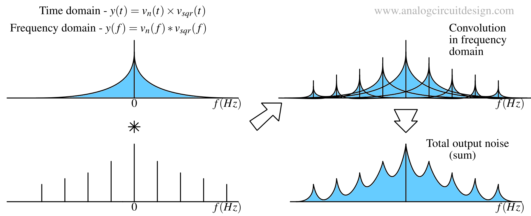
Cyclostationary Noise
If the noise vary in a periodic fashion, the noise is said to be a cyclostationary noise1. Stationary means time-invariant. In real circuits, cyclostationarity arises when a time-varying operating point modulates the noise produced by bias-dependent noise sources (e.g., Gilbert mixers), or when the time-varying nature of the circuit alters the transfer function from the noise source to the output (e.g., sample and hold circuits, passive mixers).
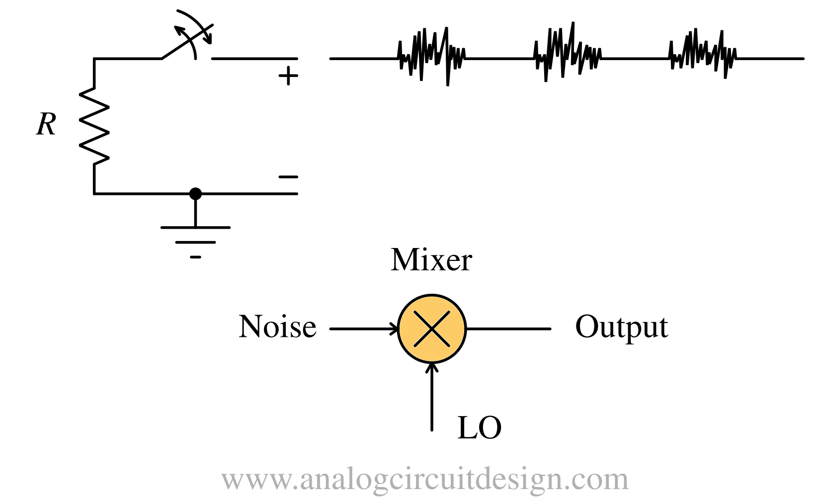
The above illustration shows a simple example of cyclostationary noise. A switch opening and closing periodically between the noisy resistor and the ground causes the output noise to have periodically varying statistics. Noise is transmitted from the resistor to the output only when the switch is closed.
-
Noise in mixers, oscillators, samplers, and logic an introduction to cyclostationary noise ↩
-
T. H. Lee and A. Hajimiri, "Oscillator phase noise: a tutorial," in IEEE Journal of Solid-State Circuits, vol. 35, no. 3, pp. 326-336, March 2000, doi: 10.1109/4.826814. ↩
-
D. Ham and A. Hajimiri, "Concepts and methods in optimization of integrated LC VCOs," in IEEE Journal of Solid-State Circuits, vol. 36, no. 6, pp. 896-909, June 2001, doi: 10.1109/4.924852. ↩