Second order systems
A second-order system is a dynamic system described by a second-order ordinary differential equation (ODE), often found in electrical applications like RLC circuits, filters, opamps, negative feedback circuits etc. Higher-order systems are frequently simplified or approximated to second-order systems. These systems are the simplest to show oscillatory responses, and their step response provides key transient features such as rise time, overshoot, settling time, and damping characteristics.
Second order system analysis online tool
Second order system block diagram
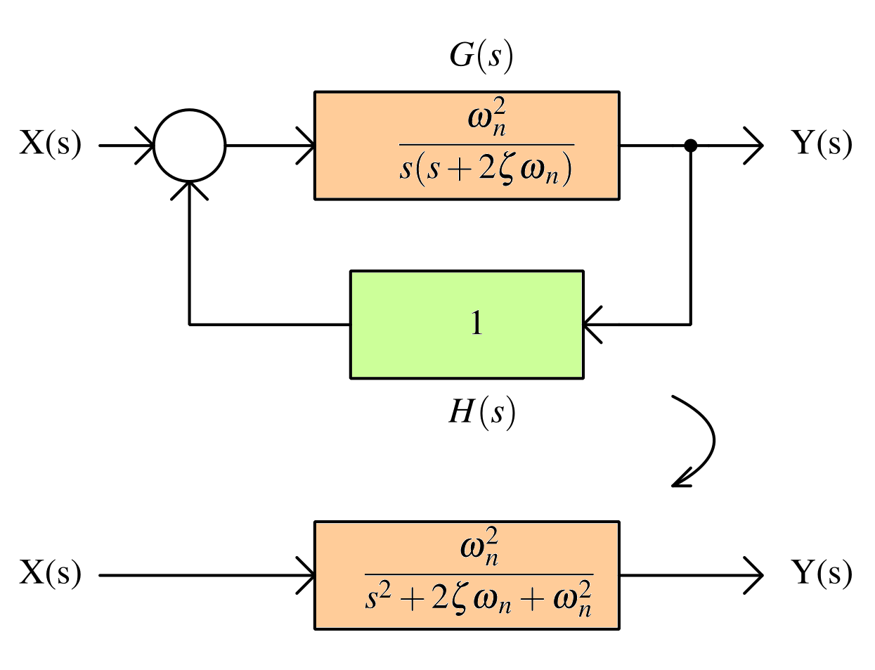
The advantage of above system is that it represents most commonly occuring control systems in use. A very common example is operational amplifiers which are modelled as second order system having two key properties related to control systems:
- Gain bandwidth product
- Phase margin
Second order system transfer function
The general equation of the transfer function of second order control system is given as :
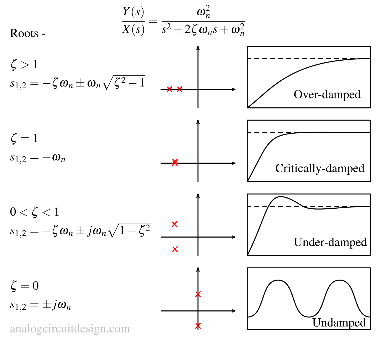
$$T(s)=\cfrac{Y(s)}{X(s)}=\cfrac{G(s)}{1+G(s)H(s)}=\cfrac{\omega{}_n^2}{s^2+2\zeta{}\omega{}_ns+\omega{}_n^2}$$
Roots of the second order system
The characteristics equation is - $$s^2+2\zeta{}\omega{}_ns+\omega{}_n^2=0$$ The roots of characteristic equation are - $$s=\cfrac{-2\omega{}\zeta{}_n\pm{}\sqrt{(2\zeta{}\omega{}_n)^2-4\omega{}_n^2}}{2}=\cfrac{-2(\zeta{}\omega{}_n\pm{}\omega{}_n\sqrt{\zeta{}^2-1})}{2}$$ $$\implies{}s=-\zeta{}\omega{}_n\pm{}\omega{}_n\sqrt{\zeta{}^2-1}$$
Damping factor and natural frequency
The damping factor or damping ratio (\(\zeta{}\)) quantifies how long oscillations stay in a system after a disturbance. Values :
- \( \zeta{}<1 \): Underdamped (Oscillatory)
- \( \zeta{}=1 \): Critically damped (fastest, no oscillation)
- \( \zeta{}>1 \): Overdamped (non-oscillatory, slow)
The natural frequency (\(\omega{}_n\)) is the frequency at which a system oscillates when damping or damping factor (\(\zeta{}\)) is zero.
The damped natural frequency (\(\omega{}_d=\omega{}_n\sqrt{1-\zeta{}^2}\)). This is the frequency of oscillations as actually observed in a damped system
Impulse response of second order systems
Laplace transform of the unit step \(\delta{}(t)\) signal is 1. Therefore X(s), $$X(s)=1$$ $$T(s)=\cfrac{Y(s)}{X(s)}=\cfrac{\omega{}_n^2}{s^2+2\zeta{}\omega{}_ns+\omega{}_n^2}$$
Underdamped
When \(0\leq{}\zeta{}<1\),
$$y(t)=\cfrac{1}{\sqrt{1-\zeta{}^2}}e^{-\zeta{}\omega{}_nt}\sin{\left(\omega{}_n\sqrt{1-\zeta{}^2}t+\phi{}\right)}$$
The response settles to zero after some oscillation
Derivation of underdamped impulse response
When \(0\leq{}\zeta{}<1\), the characteristic equation can be rewritten as (to easily convert into inverse laplace): $$s^2+2\zeta{}\omega{}_ns+\omega{}_n^2=\left[s^2+2(s)(\zeta{}\omega{}_n)+(\zeta{}\omega{}_n)^2\right]+\left[\omega{}_n^2-\zeta{}^2\omega{}_n^2\right]$$ $$=(s+\zeta{}\omega_n)^2+\omega_n^2(1-\zeta{}^2)$$ The transfer function becomes, $$\cfrac{Y(s)}{X(s)}=\cfrac{\omega{}_n^2}{(s+\zeta{}\omega{}_n)^2+\omega{}_n^2(1-\zeta{}^2)}$$ Substituting \(X(s)=1\), $$Y(s)=\cfrac{\omega{}_n^2}{(s+\zeta{}\omega{}_n)^2+\omega{}_n^2(1-\zeta{}^2)}X(s)=\cfrac{\omega{}_n^2}{(s+\zeta{}\omega{}_n)^2+\omega{}_n^2(1-\zeta{}^2)}$$ Taking inverse Laplace transform (assuming zero initial conditions), $$y(t)=\cfrac{1}{\sqrt{1-\zeta{}^2}}e^{-\zeta{}\omega{}_nt}\sin{\left(\omega{}_n\sqrt{1-\zeta{}^2}t+\phi{}\right)}$$
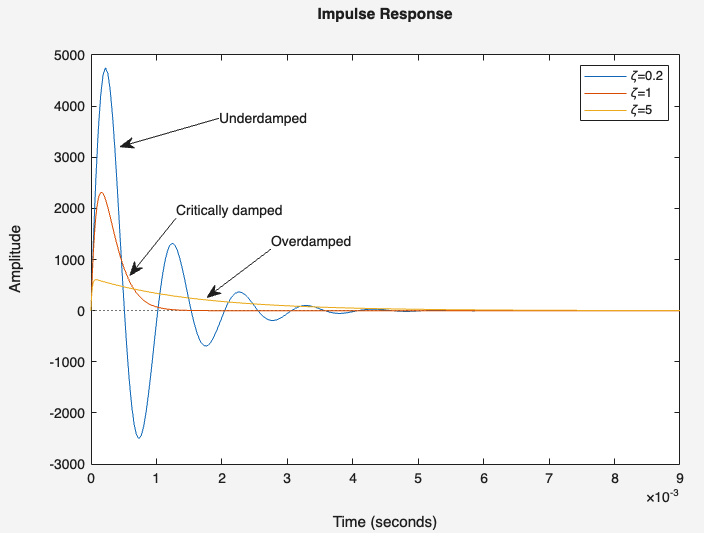
Critically damped
When \(\zeta{}=1\), $$y(t)=te^{-\omega{}_nt}u(t)$$ The response will reach the step input in steady state without oscillations or overshoot.
Derivation of critically damped
When \(\zeta{}=1\), the characteristic equation becomes: $$T(s)=\cfrac{Y(s)}{X(s)}=\cfrac{\omega{}_n^2}{s^2+2\omega{}_ns+\omega{}_n^2}=\cfrac{\omega{}_n^2}{(s+\omega{}_n)^2}$$ $$\implies{}Y(s)=\cfrac{\omega{}_n^2}{(s+\omega{}_n)^2}X(s)$$ Substituting \(X(s)=1\), $$Y(s)=\cfrac{\omega{}_n^2}{(s+\omega{}_n)^2}$$ Applying inverse laplace transform (assuming zero initial conditions), $$y(t)=te^{-\omega{}_nt}u(t)$$
Overdamped
When \(\zeta{}>1\),
$$y(t)=\cfrac{1}{2\omega{}_n\sqrt{\zeta{}^2-1}}\left(e^{-(\zeta{}\omega{}_n-\omega{}_n\sqrt{\zeta{}^2-1})t}-e^{-(\zeta{}\omega{}_n+\omega{}_n\sqrt{\zeta{}^2-1})t}\right)u(t)$$
The response reaches the unit step after infinite time.
Derivation of overdamped system
When \(\zeta{}>1\), the characteristic equation can be rewritten as : $$s^2+2\zeta{}\omega{}_ns+\omega{}_n^2=(s+\zeta{}\omega{}_n)^2-\omega{}_n^2(\zeta{}^2-1)$$
The transfer function becomes, $$\cfrac{Y(s)}{X(s)}=\cfrac{\omega_n^2}{(s+\zeta{}\omega_n)^2-\omega_n^2(\zeta{}^2-1)}$$ Substituting \(X(s)=1\), $$Y(s)=\cfrac{\omega{}_n^2}{(s+\zeta{}\omega{}_n)^2-\omega{}_n^2(\zeta{}^2-1)}X(s)=\cfrac{\omega{}_n^2}{(s+\zeta{}\omega{}_n)^2-\omega{}_n^2(\zeta{}^2-1)}$$
Taking inverse Laplace transform (assuming zero initial conditions), $$y(t)=\cfrac{1}{2\omega{}_n\sqrt{\zeta{}^2-1}}\left(e^{-(\zeta{}\omega{}_n-\omega{}_n\sqrt{\zeta{}^2-1})t}-e^{-(\zeta{}\omega{}_n+\omega{}_n\sqrt{\zeta{}^2-1})t}\right)u(t)$$
Step response of second order systems
Laplace transform of the unit step \(u(t)\) signal is \(1/s\). Therefore X(s), $$X(s)=\cfrac{1}{s}$$ $$T(s)=\cfrac{Y(s)}{X(s)}=\cfrac{\omega{}_n^2}{s^2+2\zeta{}\omega{}_ns+\omega{}_n^2}$$
Underdamped
When \(0\leq{}\zeta{}<1\), $$y(t)=1-\cfrac{e^{-\zeta{}\omega{}_nt}}{\sqrt{1-\zeta{}^2}}\sin\left[\left(\omega{}_n\sqrt{1-\zeta{}^2}\right)t+\phi{}\right]$$ Where, $$\phi{}=\tan{}^{-1}\cfrac{\sqrt{1-\zeta{}^2}}{\zeta{}}$$ The unit step response settles to the step function with decaying oscillations when \(\zeta{}\) lies between zero and one. The frequency of oscillation is \(\omega{}_d\) and the time constant of exponential decay is \(1/\zeta{}\omega{}_n\). Where \(\omega{}_d\) is referred as damped frequency and \(\omega{}_n\) is the natural frequency.
Derivation of underdamped step response
When \(0\leq{}\zeta{}<1\), the characteristic equation can be rewritten as (to easily convert into inverse laplace): $$s^2+2\zeta{}\omega{}_ns+\omega{}_n^2=\left[s^2+2(s)(\zeta{}\omega{}_n)+(\zeta{}\omega{}_n)^2\right]+\left[\omega{}_n^2-\zeta{}^2\omega{}_n^2\right]$$ $$=(s+\zeta{}\omega_n)^2+\omega_n^2(1-\zeta{}^2)$$
The transfer function becomes, $$\cfrac{Y(s)}{X(s)}=\cfrac{\omega{}_n^2}{(s+\zeta{}\omega{}_n)^2+\omega{}_n^2(1-\zeta{}^2)}$$ Substituting \(X(s)=1/s\), $$Y(s)=\cfrac{\omega{}_n^2}{(s+\zeta{}\omega{}_n)^2+\omega{}_n^2(1-\zeta{}^2)}X(s)=\cfrac{\omega{}_n^2}{(s+\zeta{}\omega{}_n)^2+\omega{}_n^2(1-\zeta{}^2)}\cfrac{1}{s}$$
Using partial fractions we obtain, $$Y(s)=\cfrac{1}{s}-\cfrac{s+\zeta{}\omega{}_n}{(s+\zeta{}\omega{}_n)^2+\omega{}_n^2(1-\zeta{}^2)}-\cfrac{\zeta{}\omega{}_n}{(s+\zeta{}\omega{}_n)^2+\omega{}_n^2(1-\zeta{}^2)}$$ $$Y(s)=\cfrac{1}{s}-\cfrac{s+\zeta{}\omega{}_n}{(s+\zeta{}\omega{}_n)^2+\omega{}_n^2(1-\zeta{}^2)}-\cfrac{\zeta{}}{\sqrt{1-\zeta{}^2}}\cfrac{\omega{}_n\sqrt{1-\zeta{}^2}}{(s+\zeta{}\omega{}_n)^2+\omega{}_n^2(1-\zeta{}^2)}$$
Replacing \(\omega{}_n{}\sqrt{1-\zeta{}^2}\) with \(\omega{}_d\), $$Y(s)=\cfrac{1}{s}-\frac{(s+\zeta{}\omega{}_n)}{(s+\zeta{}\omega{}_n)^2+\omega{}_d^2}-\frac{\zeta{}}{\sqrt{1-\zeta{}^2}}\left(\frac{\omega{}_d}{(s+\zeta{}\omega{}_n)^2+\omega{}_d^2}\right)$$
Taking inverse Laplace (assuming zero initial conditions), $$y(t)=\left(1-e^{-\zeta{}\omega{}_nt}\cos(\omega{}_dt)-\cfrac{\zeta{}}{\sqrt{1-\zeta{}^2}}e^{-\zeta{}\omega{}_nt}\sin(\omega{}_dt)\right)u(t)$$
or,
$$y(t)=1-\cfrac{e^{-\zeta{}\omega{}_nt}}{\sqrt{1-\zeta{}^2}}\sin\left[\left(\omega{}_n\sqrt{1-\zeta{}^2}\right)t+\phi{}\right]$$
Where, $$\phi{}=\tan{}^{-1}\cfrac{\sqrt{1-\zeta{}^2}}{\zeta{}}$$
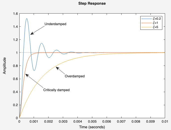
Critically damped
When \(\zeta{}=1\), the characteristic equation becomes: $$T(s)=\cfrac{Y(s)}{X(s)}=\cfrac{\omega{}_n^2}{s^2+2\omega{}_ns+\omega{}_n^2}=\cfrac{\omega{}_n^2}{(s+\omega{}_n)^2}$$ $$\implies{}Y(s)=\cfrac{\omega{}_n^2}{(s+\omega{}_n)^2}X(s)$$ Substituting \(X(s)=1/s\), $$Y(s)=\cfrac{\omega{}_n^2}{(s+\omega{}_n)^2}\cfrac{1}{s}$$ Using partial fractions, $$Y(s)=\cfrac{1}{s}-\cfrac{1}{s+\omega{}_n}-\frac{\omega{}_n}{(s+\omega{}_n)^2}$$ Applying inverse laplace transform (assuming zero initial conditions), $$y(t)=(1-\underbrace{e^{-\omega{}_nt}-\omega{}_nte^{-\omega{}_nt}}_{\rightarrow{}0})u(t)$$
The response will reach the step input in steady state without oscillations or overshoot.
Overdamped
When \(\zeta{}>1\), the characteristic equation can be rewritten as : $$s^2+2\zeta{}\omega{}_ns+\omega{}_n^2=(s+\zeta{}\omega{}_n)^2-\omega{}_n^2(\zeta{}^2-1)$$
The transfer function becomes, $$\cfrac{Y(s)}{X(s)}=\cfrac{\omega_n^2}{(s+\zeta{}\omega_n)^2-\omega_n^2(\zeta{}^2-1)}$$ Substituting \(X(s)=1/s\), $$Y(s)=\cfrac{\omega{}_n^2}{(s+\zeta{}\omega{}_n)^2-\omega{}_n^2(\zeta{}^2-1)}X(s)=\cfrac{\omega{}_n^2}{(s+\zeta{}\omega{}_n)^2-\omega{}_n^2(\zeta{}^2-1)}\cfrac{1}{s}$$
Using partial fractions we obtain, $$Y(s)=\cfrac{1}{s}+\cfrac{1}{2(\zeta{}+\sqrt{\zeta{}^2-1})(\sqrt{\zeta{}^2-1})}\cfrac{1}{s+\zeta{}\omega{}_n+\omega{}_n\sqrt{(\zeta{}^2-1)}}-\cfrac{1}{2(\zeta{}-\sqrt{\zeta{}^2-1})(\sqrt{\zeta{}^2-1})}\cfrac{1}{s+\zeta{}\omega{}_n-\omega{}_n\sqrt{(\zeta{}^2-1)}}$$
Taking inverse Laplace transform (assuming zero initial conditions), $$y(t)=\left(1+\left(\cfrac{1}{2(\zeta{}+\sqrt{\zeta{}^2-1})(\sqrt{\zeta{}^2-1})}\right)e^{-(\zeta{}\omega{}_n+\omega{}_n\sqrt{\zeta{}^2-1})t}-\left(\cfrac{1}{2(\zeta{}-\sqrt{\zeta{}^2-1})(\sqrt{\zeta{}^2-1})}\right)e^{-(\zeta{}\omega{}_n-\omega{}_n\sqrt{\zeta{}^2-1})t}\right)u(t)$$
The response reaches the unit step after infinite time.
Parameters in step response
Delay time
In a second-order system, the delay time (\(t_d\)) is the time required for the system’s step response to reach 50% of its final value for the first time. $$t_d=\cfrac{1+0.7\zeta{}}{\omega{}_n}$$
Rise time
The rise time \(t_r\) is defined as the time the step response takes to rise from 10% to 90% (sometimes 0% to 100%) of its final value. It is a key measure of how quickly the system responds. $$t_r=\cfrac{\pi{}-\tan{}^{-1}\cfrac{\sqrt{1-\zeta{}^2}}{\zeta{}}}{\omega{}_n\sqrt{1-\zeta{}^2}}$$
Derivation of Rise time
The magnitude of output signal at rise time is 1. Basically it is the time when output hits the steady state value for the first time. After this, it overshoots and takes settling time to become steady. $$1=1-e^{-\zeta{}\omega{}_nt_r}\cos(\omega{}_dt_r)-\cfrac{\zeta{}}{\sqrt{1-\zeta{}^2}}e^{-\zeta{}\omega{}_nt_r}\sin(\omega{}_dt_r)$$ $$e^{-\zeta{}\omega{}_nt_r}\cos(\omega{}_dt_r)-\cfrac{\zeta{}}{\sqrt{1-\zeta{}^2}}e^{-\zeta{}\omega{}_nt_r}\sin(\omega{}_dt_r)=0$$ $$\cos(\omega{}_dt_r)-\cfrac{\zeta{}}{\sqrt{1-\zeta{}^2}}\sin(\omega{}_dt_r)=0$$ The left hand side can be written as : $$\cos(\omega{}_dt_r)-\cfrac{\zeta{}}{\sqrt{1-\zeta{}^2}}\sin(\omega{}_dt_r)=\sin\left[\left(\omega{}_n\sqrt{1-\zeta{}^2}\right)t_r+\phi{}\right]$$ Where, $$\phi{}=\tan{}^{-1}\cfrac{\sqrt{1-\zeta{}^2}}{\zeta{}}$$ $$\implies{}\sin\left[\left(\omega{}_n\sqrt{1-\zeta{}^2}\right)t_r+\phi{}\right]=0$$ $$\implies{}t_r=\cfrac{\pi{}-\phi{}}{\omega{}_n\sqrt{1-\zeta{}^2}}$$
Peak time
It is the time it takes for the step response of a system to reach its first maximum value (the peak overshoot). It indicates how quickly the system reaches its maximum excursion before settling toward the final value. $$t_p=\cfrac{\pi}{\omega{}_n\sqrt{1-\zeta{}^2}}$$
Derivation of Peak time
As per definition the response curve reaches to its maximum value at peak time. Hence at that point, $$\cfrac{dy(t)}{dt}=0$$ From above, \(y(t)\): $$y(t)=1-\cfrac{e^{-\zeta{}\omega{}_nt}}{\sqrt{1-\zeta{}^2}}\sin{\left(\omega{}_n\sqrt{1-\zeta{}^2}t+\phi{}\right)}$$ $$\cfrac{dy(t)}{dt}=-\cfrac{e^{-\zeta{}\omega{}_nt}}{\sqrt{1-\zeta{}^2}}\omega{}_n\sqrt{1-\zeta{}^2}\cos{\left(\omega{}_n\sqrt{1-\zeta{}^2}t+\phi{}\right)}-\cfrac{(-\zeta{}\omega{}_n)e^{-\zeta{}\omega{}_nt}}{\sqrt{1-\zeta{}^2}}\sin{\left(\omega{}_n\sqrt{1-\zeta{}^2}t+\phi{}\right)}$$ Putting, \(dy(t)/dt=0\) $$\therefore{}\cfrac{e^{-\zeta{}\omega{}_nt}}{\sqrt{1-\zeta{}^2}}\left(-\omega{}_n\sqrt{1-\zeta{}^2}\cos{\left(\omega{}_n\sqrt{1-\zeta{}^2}t+\phi{}\right)}+\zeta{}\omega{}_n\sin{\left(\omega{}_n\sqrt{1-\zeta{}^2}t+\phi{}\right)}\right)=0$$ $$\omega{}_n\sqrt{1-\zeta{}^2}\cos{\left(\omega{}_n\sqrt{1-\zeta{}^2}t+\phi{}\right)}=\zeta{}\omega{}_n\sin{\left(\omega{}_n\sqrt{1-\zeta{}^2}t+\phi{}\right)}$$ $$\implies{}\tan{\left(\omega{}_n\sqrt{1-\zeta{}^2}+\phi{}\right)}=\cfrac{\sqrt{1-\zeta{}^2}}{\zeta{}}=\tan{\phi{}}$$ $$\therefore{}\left(\omega{}_n\sqrt{1-\zeta{}^2}\right)t=n\pi{}$$ $$t_p=\cfrac{\pi{}}{\omega{}_n\sqrt{1-\zeta{}^2}}$$
Maximum overshoot
The maximum overshoot \(M_p\) is the amount by which the system’s step response exceeds its final steady-state value, expressed as a percentage of that value. It represents how much the system “overreacts” before settling. $$M_p=\cfrac{y(t_p)-y(\infty)}{y(\infty)}\times{}100\%$$ $$\implies{}M_p=e^{-\zeta{}\pi{}/\sqrt{1-\zeta{}^2}}\times{}100$$
Settling time
The settling time \(t_s\) is the time required for the system’s step response to stay within a specified percentage band around its final value (typically ±2% or ±5%). It indicates how quickly the oscillations or deviations die out and response become steady.
For 2% criterion, $$t_s=\cfrac{4}{\zeta{}\omega{}_n}$$
For 5% criterion, $$t_s=\cfrac{3}{\zeta{}\omega{}_n}$$
Steady-state error
Steady state error is the difference between actual output and desired output after long time.
$$e_{ss}=\lim_{t\to\infty}e(t)=\lim_{t\to\infty}[y(t)-x(t)]$$
Second order system examples
- A simple RLC (resistor, inductor, capacitor) circuit, whether series or parallel, is a classic example. The inductor and capacitor both store energy, making it a second-order system.
- A servo system, used for position control, is often a second-order system. It involves components like a proportional controller and load elements.
- A PLL is a control system that controls a voltage-controlled oscillator (VCO) to match a reference frequency. The VCO acts as an integrator, leading to a second-order system.
- An operational amplifier in negative feedback is a second order system. The operational amplifier has a dominant and non-dominant pole.
Second order bode plot
The bode plot reveals critical information about a second order system such as phase and gain margin. This information can be used to determine the stability of a system. It indicates how a step response would look like.
Second order system analysis using Matlab
Step response
    %% Second order system step response
    %% Defining the natural frequency
    wn = 2*pi*1000;
    %% Defining the damping factor
    zeta = 0.2;
    num = wn^2;
    den = [1 2*zeta*wn wn^2];
    sys = tf(num,den);
    step(sys);

    zeta = 1;
    num = wn^2;
    den = [1 2*zeta*wn wn^2];
    sys = tf(num,den);
    hold on;
    step(sys);

    zeta = 5;
    num = wn^2;
    den = [1 2*zeta*wn wn^2];
    sys = tf(num,den);
    hold on;
    step(sys);
Bode plot
    %% Open loop system
    zeta = 0.2;
    num = wn^2;
    den = [1 zeta*wn 0];
    sys = tf(num,den);
    bp=bodeplot(sys,{1,100000});
    bp.FrequencyUnit = "Hz";
    grid on;

    %% Closed loop system with beta=1
    figure;
    bp=bodeplot(sys/(1+sys),{1,100000});
    bp.FrequencyUnit = "Hz";
    grid on;
    figure;
    step(sys/(1+sys));