State space analysis
State-space analysis is a modern approach to control system engineering that represents a physical system as a set of first-order differential equations. Unlike the classical "Transfer Function" approach (which only looks at Input vs. Output), state-space analysis looks inside the system to see what its internal variables are doing.
State space representation
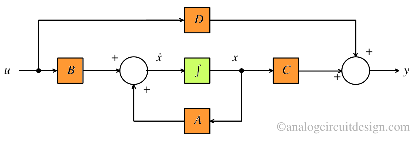
$$\dot{x}=Ax+Bu$$ $$y=Cx+Du$$ Here \(\dot{x}=dx/dt\). The first equation is called State equation. The second equation is called Output equation.
| System Type | State-space model | Laplace transform | z-transform |
|---|---|---|---|
| Continous Time-Invariant | $$\dot{x}=Ax(t)+Bu(t)$$ $$y(t)=Cx(t)+Du(t)$$ | $$sX(s)-sX(0)=AX(s)+BU(s)$$ $$Y(s)=CX(s)+DU(s)$$ | - |
| Discrete Time-Invariant | $$x(n+1)=Ax(n)+Bu(n)$$ $$y(n)=Cx(n)+Du(n)$$ | - | $$zX(z)-zX(0)=AX(z)+BU(z)$$ $$Y(z)=CX(z)+DU(z)$$ |
Need for state-space analysis
Using the state-space method, one can perform the analysis and design of the following types of systems:
- Linear and non-linear systems
- Time varying and time invariant systems
- SISO (Single input and single output) systems
- MIMO (Multiple input and multiple output) systems
State-space analysis is well suited for analysis using digital computers. In contrast, conventional methods rely on the system’s transfer function. However, the transfer function approach has certain limitations, such as:
- Transfer function is defined under zero initial conditions.
- Transfer function is applicable to linear time invariant systems only.
- Transfer function analysis is restricted to single input and single output systems (SISO).
- Does not provides information regarding the internal state of the system.
Concept of state, state variables, state vector, state space
State space analysis for system with initial conditions
The output not only depends on the input applied to the system for t > t0, but also on the initial conditions at time t = t0,
$$y(t)=y(t)|_{t=t_0}+y(t)|_{t\geq{}t_0}$$
$$=\int^{t_0}_{-\infty{}}y(t)+\int^{t}_{t_0}y(t)$$
$$=y(t_0)+\int^t_0y(t)$$
State
It is a group of variables, which summarizes the history of the system in order to predict the future values (outputs). The term \(y(t_0)\) is called the state of the system.
State variables
The variable that represents this state of the system is called the state variable. The number of the state variables required is equal to the number of the storage elements present in the system. Examples − current flowing through inductor, voltage across capacitor.
In state-space modeling of the systems, the choice of state variables is arbitrary. One of the possible choice is physical variables. The state equations are obtained from the differential equations governing the system.
State vector
It is a vector, which contains the state variables as elements. There are two mathematical models of a control systems. Differential equation model and the transfer function model. The state space model can be obtained from any one of these two mathematical models. $$\dot{X(t)}=\begin{bmatrix}x_1(t) \\ x_2(t) \\ \vdots{} \\ x_n(t)\end{bmatrix}$$
Selection of state variables
The state variables of a system are not unique; multiple valid choices can represent the same system.
- In a physical system, the required number of state variables equals the number of energy-storing elements in the system.
- For a system described by a linear constant-coefficient differential equation, the number of state variables equals the order of the differential equation.
- For a system represented by a transfer function, the number of state variables equals the highest power of \(s\) in the denominator of the transfer function.
Formulation of state space
State-space analysis uses a set of first-order differential or difference equations to represent a dynamic system, to describe how the system's internal states evolve over time and an output equation that relates the states to observable outputs.
Consider a multi-input & multi-output system is having:
- m inputs : \(u_1(t), u_2(t) \dots{} u_m(t)\)
- p outputs : \(y_1(t), y_2(t) \dots{} y_p(t) \)
- n state variables : \(x_1(t), x_2(t) \dots{} x_n(t)\)
Different variables may be represented by the vectors as shown below:
Input vector
$$U(t)=\begin{bmatrix}u_1(t) \\ u_2(t) \\ \vdots{} \\ u_m(t)\end{bmatrix}$$
Output vector
$$Y(t)=\begin{bmatrix}y_1(t) \\ y_2(t) \\ \vdots{} \\ y_p(t)\end{bmatrix}$$
State variable vector
$$\dot{X(t)}=\begin{bmatrix}x_1(t) \\ x_2(t) \\ \vdots{} \\ x_n(t)\end{bmatrix}$$
The state-variable representation can be expressed as a set of n first-order differential equations, as shown below:
$$\cfrac{dx_1}{dt}=\dot{x_1}=a_{11}x_1+a_{12}x_2\dots{}a_{1n}x_n + b_{11}u_1+b_{12}u_2\dots{}b_{1m}u_m$$
$$\cfrac{dx_2}{dt}=\dot{x_2}=a_{21}x_1+a_{22}x_2\dots{}a_{2n}x_n + b_{21}u_1+b_{22}u_2\dots{}b_{2m}u_m$$
$$\dots{}$$
$$\dots{}$$
$$\cfrac{dx_n}{dt}=\dot{x_n}=a_{n1}x_1+a_{n2}x_2\dots{}a_{nn}x_n + b_{n1}u_1+b_{n2}u_2\dots{}b_{nm}u_m$$
Where coefficients \(a_{ij}\) and \(b_{ij}\) are constants.
In Matrix form, $$\begin{bmatrix}\dot{x_1} \\ \dot{x_2} \\ \vdots{} \\ \dot{x_n}\end{bmatrix}=\begin{bmatrix}a_{11} & \dots{} & a_{1n} \\ a_{21} & \dots{} & a_{2n} \\ \vdots{} \\ a_{n1} & \dots{} & a_{nn} \end{bmatrix} \begin{bmatrix}x_1 \\ x_2 \\ \vdots{} \\ x_n\end{bmatrix}+\begin{bmatrix}b_{11} & \dots{} & b_{1n} \\ b_{21} & \dots{} & b_{2n} \\ \vdots{} \\ b_{n1} & \dots{} & b_{nn} \end{bmatrix} \begin{bmatrix}u_1 \\ u_2 \\ \vdots{} \\ u_m\end{bmatrix}$$
The above equation can be represented as : $$\dot{X(t)}=AX(t)+BU(t)$$
The above equation is called state equation.
Output equation
The output at any time are functions of state variables and inputs. The outputs can be expressed as a linear combination of state variables and inputs.
$$y_1=c_{11}x_1+c_{12}x_2\dots{}c_{1n}x_n + d_{11}u_1+d_{12}u_2\dots{}d_{1m}u_m$$
$$y_2=c_{21}x_1+c_{22}x_2\dots{}c_{2n}x_n + d_{21}u_1+d_{22}u_2\dots{}d_{2m}u_m$$
$$\dots{}$$
$$\dots{}$$
$$y_p=c_{p1}x_1+c_{p2}x_2\dots{}c_{pn}x_n + d_{p1}u_1+d_{p2}u_2\dots{}d_{pm}u_m$$
Where coefficients \(c_{ij}\) and \(d_{ij}\) are constants.
In the matrix form,
$$\begin{bmatrix}y_1 \\ y_2 \\ \vdots{} \\ y_n\end{bmatrix}=\begin{bmatrix}c_{11} & \dots{} & c_{1n} \\ c_{21} & \dots{} & c_{2n} \\ \vdots{} \\ c_{p1} & \dots{} & c_{pn} \end{bmatrix} \begin{bmatrix}x_1 \\ x_2 \\ \vdots{} \\ x_n\end{bmatrix}+\begin{bmatrix}d_{11} & \dots{} & d_{1n} \\ d_{21} & \dots{} & d_{2n} \\ \vdots{} \\ d_{p1} & \dots{} & b_{pn} \end{bmatrix} \begin{bmatrix}u_1 \\ u_2 \\ \vdots{} \\ u_m\end{bmatrix}$$
The above equation can be represented as : $$y(t)=CX(t)+DU(t)$$
The above equation is called output equation.
Laplace transform of state space equations
State space equations :
$$\cfrac{dx}{dt}=Ax+Bu\hspace{0.2in}(\text{State equation})$$
$$y=Cx+Du\hspace{0.2in}(\text{Output equation})$$
Derivation
Applying Laplace Transform in both the sides, $$sX(s)=AX(s)+BU(s)$$ $$\implies{}(sI-A)X(s)=BU(s)$$ $$X(s)=(sI-A)^{-1}BU(s)$$ Applying Laplace Transform on both sides of output equation. $$Y(s)=CX(s)+DU(s)$$ Substitute, X(s) value in the above equation. $$\implies{}Y(s)=C(sI-A)^{-1}BU(s)+DU(s)$$ $$\implies{}Y(s)=\left[C(sI-A)^{-1}BU(s)+D\right]U(s)$$
$$\cfrac{Y(s)}{U(s)}=C\left(sI-A\right)^{-1}B+D$$
Example of State Space to Laplace Transform
$$\dot{X}=\begin{bmatrix}\dot{x}_1 \\ \dot{x}_2 \end{bmatrix}=\begin{bmatrix}-1 & -1 \\1 & 0 \end{bmatrix}\begin{bmatrix}x_1 \\x_2 \end{bmatrix}+\begin{bmatrix}1 \\0 \end{bmatrix}[u]$$ $$Y=\begin{bmatrix}0 & 1 \end{bmatrix}\begin{bmatrix}x_1 \\x_2 \end{bmatrix}$$ Here, $$A=\begin{bmatrix}-1 & -1 \\1 & 0 \end{bmatrix}, \quad B=\begin{bmatrix}1 \\0 \end{bmatrix}, \quad C=\begin{bmatrix}0 & 1 \end{bmatrix} \quad \text{and} \quad D=[0]$$
The formula for the transfer function when D=[0] is -
$$\cfrac{Y(s)}{U(s)}=C\left(sI-A\right)^{-1}B$$
Substitute A, B, C matrices in the above equation.
$$\cfrac{Y(s)}{U(s)}=\begin{bmatrix}0 & 1 \end{bmatrix}\begin{bmatrix}s+1 & 1 \\ -1 & s \end{bmatrix}^{-1}\begin{bmatrix}1 \\0 \end{bmatrix}$$
$$\Rightarrow \frac{Y(s)}{U(s)}=\begin{bmatrix}0 & 1 \end{bmatrix} \frac{\begin{bmatrix}s & -1 \\1 & s+1 \end{bmatrix}}{(s+1)s-1(-1)}\begin{bmatrix}1 \\0 \end{bmatrix}$$
$$\Rightarrow \frac{Y(s)}{U(s)}=\begin{bmatrix}0 & 1 \end{bmatrix} \frac{\begin{bmatrix}s & -1 \\1 & s+1 \end{bmatrix}}{(s+1)s-1(-1)}\begin{bmatrix}1 \\0 \end{bmatrix}=\cfrac{1}{s^2+s+1}$$
State Space Model from Differential Equation
To transform a differential equation into a state-space model, define state variables, typically as the system's energy storage elements and derivatives, and then write the system dynamics as a set of first-order differential equations (state equations) and an output equation relating outputs to these states and inputs.
Identify State Variables
Choose a minimal set of state variables that fully describe the system's current state and are required to predict its future behavior. For physical systems, these are often the energy storage elements and their derivatives (e.g., position and velocity for a mass-spring system, or capacitor voltage and inductor current for an RLC circuit).
Write First-Order Differential Equations:
- For each state variable, write its derivative
- For a higher-order differential equation, introduce a new state variable for each order. This converts the higher-order equation into a system of coupled first-order equations.
Formulate State Equations
Arrange these first-order differential equations into the standard matrix form: $$\dot{x}=Ax(t)+Bu(t)$$ Where:
- \(\dot{x}\) is the vector of the time derivatives of the state variables.
- \(x(t)\) is the state vector.
- \(u(t)\) is the input vector.
- A is the system matrix, derived from the coefficients of the state variables in the state equations.
- B is the input matrix, derived from the coefficients of the input in the state equations.
Formulate the Output Equation:
Define the system's outputs (y(t)) as a linear combination of the state variables and inputs.
$$y(t) = Cx(t) + Du(t)$$
Where:
- C is the output matrix, derived from the relationships between the state variables and the output.
- D is the feed-forward matrix, representing the direct influence of the input on the output.
Controllability
A system is completely controllable if the initial state of the system is transferred to any particular state, in a finite time duration, when a controlled input is provided to it.
Kalmans test
Create the composite matrix Mc as shown below :
$$M_c=[B\hspace{0.2in}AB\hspace{0.2in}A^2B\hspace{0.2in}\dots{}\hspace{0.2in}A^{n-1}B]$$
Find the determinant of composite matrix Mc and if it is not equal to zero, then the control system is controllable.
Necessary and sufficient condition to check controllability
$$\text{rank}\,M_c=\text{rank}\,[B\hspace{0.2in}AB\hspace{0.2in}A^2B\hspace{0.2in}\dots{}\hspace{0.2in}A^{n-1}B]=n$$
Observability
Observability of a control system is the ability of the system to determine the internal states of the system by observing the output in a finite time interval when input is provided to the system. It is another crucial property of the control system as it shows the behavioural approach of the control system.
Kalmans test
Write the matrix \(M_o\) in following form :
$$M_o=[C^T\hspace{0.2in}A^TC^T\hspace{0.2in}(A^T)^2C^T\hspace{0.2in}\dots{}\hspace{0.2in}(A^T)^{n-1}C^T]$$
If the determinant of the matrix Mo is not zero, then the control system is observable.