Negative feedback Systems
A closed-loop negative feedback control system (or simply negative feedback system) continuously monitors the system's output and adjusts it to match the desired input, reducing the error signal to zero. This is achieved through real-time feedback, allowing the system to make automatic adjustments to maintain the desired setpoint. In contrast, a closed-loop positive feedback system increases the error signal and has a different application.
Closed loop negative feeback system block diagram

Key elements of a closed-loop feedback system include:
- Input: This is the signal or information that represents the desired state or setpoint for the system. It specifies the goal or the behavior that the control system aims to achieve.
- Difference block (comparator or summer): This block compares the input and feedback signal (a scaled copy of output) and generates an error signal. For example, in an operational amplifier, the function of difference block is achieved by a differential pair.
- Controller: Controller takes the error signal generated from the comparator/difference-block and generates a control action or command to bring the system closer to the desired state. Controllers can be implemented using various algorithms, including proportional-integral-derivative (PID) controllers, state-space controllers, and more. For example, in an operational-amplifier, it is the transconductance and compensation network.
- Plant (Process): The plant, often referred to as the system or process, is the physical or mathematical representation of the system being controlled. It could be a machine, a chemical process, an electrical circuit, or any other dynamic system that requires regulation. In an op-amp, the output stage is considered as the plant. In motor drive applications, large MOSFETs are used to drive the motors which can be considered as the plant.
- Output: The output is the response of the plant to the control action generated by the controller. It represents the actual behavior of the system at any given time.
- Feedback sensors: Feedback is the process of measuring the output of the system and comparing it to the desired input (setpoint). The controller makes adjustments to the control action to minimize the difference between the desired and actual states based on the output of the feedback sensor. In an op-amp, it the feedback β-network which can be considered as sensors. The input of the β network is voltage and output is also voltage.
Mathematical representation (transfer function) of a closed loop negative feedback system

To find the transfer function y(s)/x(s) of the above system, we shall list the simple relations below:
$$e(s)=x(s)-f(s)$$
$$u(s)=e(s)\cdot{}K(s)$$
$$y(s)=u(s)\cdot{}G(s)$$
$$f(s)=y(s)\cdot{}H(s)$$
After solving the above equations, we can find the transfer function :
$$\implies{}\cfrac{y(s)}{x(s)}=\cfrac{K(s)G(s)}{1+K(s)G(s)H(s)}$$
Operational amplifier model
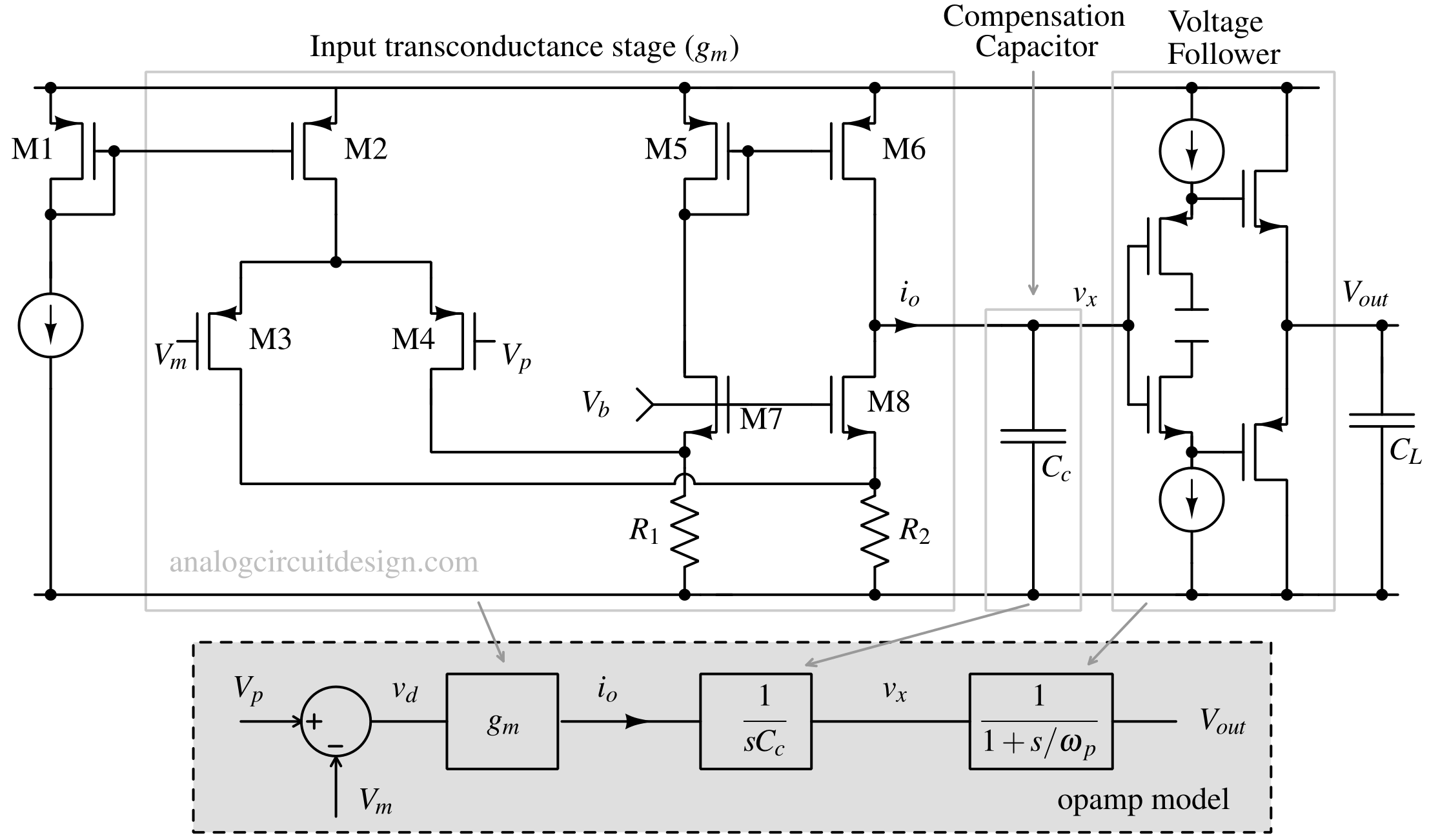
An operational amplifier is usually modeled as shown above for transient stability analysis. The input stage of an operational amplifier is a transconductor stage (or VCCS) having infinite DC gain, which has been modeled as gm stage. The output is a current io.
$$i_o=g_m(V_p-V_m)=g_mV_d$$
In the above relation, Vd=Vp-Vm. The output current (io) goes into a compensation capacitor, creating a voltage (vx). The transfer function of the compensation capacitor is (1/sCc).
$$v_x=i_o\times{}\cfrac{1}{sC_c}$$
Controller
Substituting io from above equations, we get the voltage at node vx:
$$\cfrac{v_x}{v_d}=g_m\times{}\cfrac{1}{sC_c}=\cfrac{g_m}{sC_c}=K(s)$$
The output stage transfer function is modeled as a unity gain amplifier with a pole at ωp. At DC, the gain is unity and beyond frequency greater than ωp, gain starts falling. The transfer function of the output stage is :
$$\cfrac{v_o}{v_x}=\cfrac{1}{1+\cfrac{s}{\omega{}_p}}=G(s)$$
Therefore, the overall transfer function from vd to vo is :
$$\cfrac{v_o}{v_d}=\cfrac{v_x}{v_d}\times{}\cfrac{v_o}{v_x}=\cfrac{g_m}{sC_c}\times{}\cfrac{1}{1+\cfrac{s}{\omega{}_p}}$$
$$\implies{}\cfrac{v_o}{v_d}=\cfrac{g_m}{sC_c}\cfrac{1}{1+s/\omega{}_p}=K(s)G(s)$$
Feedback network
An opamp is mostly used in closed loop negative feedback configuration. One of such model is shown below :

In the above figure, an operational amplifier is configured in non-inverting mode. In the right side, the control system model is used which is derived earlier. The feedback factor (also called beta, β), which is nothing but transfer function from vout to vm is :
$$H(s)=\beta{}=\cfrac{R_g}{R_f+R_g}$$
Servo motor model

To grasp the concept of closed-loop control, we'll use a servo motor. Servo motors commonly integrate a feedback mechanism as shown above, like an encoder or a potentiometer, to capture the motor's present position and speed. This feedback data is then compared to the desired input using an electronic circuit. The difference between the desired input and the actual output is used for motor control adjustments. The ultimate goal for the feedback loop is to reduce the error (difference between desired input and actual output) to zero in a steady state.
Modeling of the plant/process (motor)
The plant produces the output. To extract the model of the DC motor, we should know the nature of the output of the plant y(s) and input to the plant u(s). The output we desire is position (not speed). Since the output is the rotation of the shaft, we shall capture the angle (θ). Basically, y(s)=θ(s) and u(s)=Vb(s).
We know the relation of output angular speed with the voltage applied (or back emf) to a DC motor:
$$\cfrac{d\theta{}}{dt}=kV_b$$
or,
$$\theta{}=\int{}kV_b\cdot{}dt$$
$$\implies{}G(s)=\cfrac{\theta{}(s)}{V_b(s)}=\cfrac{k}{s}$$
Where k is a proportionality constant dependent on motor construction. For more about the back EMF of DC motor - Back EMF of a DC motor.
Modeling of feedback (potentiometer)
The output of the feedback block is a voltage vf(s) and the input to the feedback block is an angle θ(s). Let's assume that the potentiometer can rotate from 0 to 2π radians to generate from 0 to Vref voltage. Therefore,
$$\cfrac{v_f(s)}{v_{ref}}=\cfrac{\theta{}(s)}{2\pi}$$
$$\implies{}H(s)=\cfrac{v_{f}(s)}{\theta{}(s)}=\cfrac{v_{ref}}{2\pi{}}$$
Modeling of controller
We have the freedom to choose the model of controller depending upon our requirements. If we want the steady-state error to be zero, we shall use an integrator. With this integrator and another integrator in the plant (motor), we have two integrators, which can potentially have zero-phase margins. So, we also need a proportional component in the controller.
The input of the controller is voltage (error voltage) and the output of the controller is also a voltage. So, we can model the controller as,
$$K(s)=K_p+\cfrac{K_i}{s}$$

The individual models have been placed in the blocks as shown above. The model can be analyzed using a bode plot to make it stable and tune the transient response.