Root locus plot
Root locus analysis helps us understand how the system's roots shift as we adjust the feedback system's gain. We create a graph that links all the roots of the characteristic equation for the closed-loop system, which we obtain by changing the gain. The denominator of the transfer function is also known as the characteristic equation.
Having the skill to draw root loci by hand is extremely useful for understanding computer-generated root loci and for quickly getting a rough sense of their behavior.
Why we use root locus plot?
The purpose of drawing the root locus is to see for what value of K, the roots of 1+KG(s)H(s) lies in the right half plane. This also means for what value of K, the poles of the closed-loop system lie in the right half plane.
Let's take a generic system as shown in Fig 1.

K(s) is usually a scalar frequency-independent quantity represented by K. The transfer function becomes :
$$\cfrac{y(s)}{x(s)}=\cfrac{K\cdot{}G(s)}{1+K\cdot{}G(s)\cdot{}H(s)}$$

The characteristic equation 1+KG(s)H(s) defines the stability of a closed-loop system because its roots form the poles of the closed-loop system. However, it is difficult to find the poles of the closed-loop transfer function directly without computers. Most of the time we already know the loop-gain transfer function's poles and zeros. KG(s)H(s) is the loop gain transfer function. The roots of the characteristic equation can be found using the following equation:
$$1+K\cdot{}G(s)\cdot{}H(s)=0$$
Using root locus to tune the control system
The root locus doesn't just tell us if a system is stable or unstable; it can also help us design the damping ratio (ζ) and natural frequency (ωn) of a second-order feedback system. We can draw constant ζ (from the origin and radially outwards) and constant natural frequency (ωn) lines (parallel to the σ-axis) on the graph to find the desired roots. The phase margin (overshoot) is decided alone by ζ. The settling time (speed) is decided by ζ and ωn.
This helps us calculate the right gain (K) for the controller. More advanced controller designs like lag, lead, PI, PD, and PID can also be roughly created using the root locus.
Root locus rules with example
Before writing down the rules, let's make some conventions for ease of use. Np denotes the number of poles, and Nz denotes the number of zeros.
- The number of branches in the root locus equals the count of poles (Np) in the open-loop transfer function if Np > Nz. This is usually the case because most of the systems have more poles than zeros. If Np < Nz, then the number of branches equals the count of zeros (Nz).
- The root locus begins (at K = 0) at the open-loop poles and concludes (at K = ± ∞) at the open-loop zeros or at infinity.
- The angles of the asymptotes for root locus branches ending at infinity are determined by:
$$\theta{}=\cfrac{(1+2n)\pi{}}{N_p-N_z}$$ Where, $$n=0,1,2,\dots{},(N_p-N_z-1)$$
The real-axis intercept (also called root-locus centroid) of the asymptotes is given by:
$$\sigma_c=\cfrac{\sum{}p_i-\sum{}z_i}{N_p-N_z}$$ - A point on the real axis is part of the locus if there's an odd number of open-loop poles and zeros to the right of that point. Using this rule, we can divide the real axis into two segments: one with points on the locus and the other without points on the locus. The dividing points are the real open-loop poles and zeros.
- To find where the root loci cross the jω axis, we can set s = jω in the characteristic equation, make the real and imaginary parts equal to zero, and then solve for ω and K. The ω values are the root loci intercept on the imaginary axis. Alternatively, we can use Routh-stability criteria to determine imaginary axis intercepts.
- The angle of departure (φp) of a root locus from a complex open-loop pole is given by φp = 180° + φ where φ is the net angle contribution at this pole of all other open-loop poles and zeros.
The angle of arrival (φz), of a root locus from a complex open-loop zero is given by φz = 180° - φ, where φ is the net angle contribution at this zero of all other open-loop poles and zeros. - The value of K corresponding to any point s on a root locus can be obtained using the magnitude condition or:
$$K=\cfrac{\text{product of lengths between point s to poles}}{\text{product of lengths between point s to zeros}}$$
Underlying concepts of a root locus plot
Let's represent the loop gain using a general equation and note down some observations related to it.
$$KG(s)H(s)=K\cfrac{(s+z_1)(s+z_2)\dots{}}{(s+p_1)(s+p_2)\dots{}}$$
The characteristic equation can be rewritten by substituting the above relation. To find the roots we can write:
$$1+K\cfrac{(s+z_1)(s+z_2)\dots{}}{(s+p_1)(s+p_2)\dots{}}=0$$
Starting and end point of a root locus
From the above equation, we can easily find the roots of the characteristic equation for K=0 and K=∞.
For K=0, the roots are :
$$s=-p_1,-p_2,\dots{}\hspace{0.5cm}(\text{Open-loop poles})$$
For K=∞, the roots are :
$$s=-z_1,-z_2,\dots{}\hspace{0.5cm}(\text{Open-loop zeros})$$
Fortunately, K=0 is the starting point of the root locus and K=∞ is the end-point. So, we know from what point the root locus will start and end. It will start from open loop poles and end at open loop zeros.
Asymptotes in root locus plot
Asymptotes are straight lines that merge with the root locus when roots are approaching infinity. The order of the characteristic equation is Np if Np > Nz. The order of the characteristic equation is Nz if Nz > Np.
To understand the concept, let's assume Np > Nz. The order of the characteristic equation is Np. So, for any value of K in [0,∞), the equation would have Np roots. These could be a mix of real and complex conjugate roots depending on the value of K. So, there are Np paths (or branches) of roots. Some of them merged when having identical roots. Nz number of paths will end at zeros. The remaining (Np-Nz) paths will end at infinity. So, there are Np-Nz asymptotes.
Symmetry of root locus plot
For any real system, the coefficients of the characteristic equation (stable or unstable) are always a real number. Open loop transfer function's coefficients are also always a real number.
$$1+KG(s)H(s)=a_ns^n+a_{n-1}s^{n-1}+\dots{}+a_1s+a_0$$
$$a_n,a_{n-1},\dots{},a_1,a_0 \in{}R$$
For this to happen, the poles and zeros should also be real numbers or complex conjugate pairs. Since the open-loop poles and zeros are always located symmetrically about the real axis, the root loci are always symmetrical with respect to the real axis.
Angle and magnitude condition/criteria of root locus
The characteristic equation can be re-written as:
$$K\cfrac{(s+z_1)(s+z_2)\dots{}}{(s+p_1)(s+p_2)\dots{}}=-1$$
Let's assume that "s" is the root of the above equation. We can write it in polar form (because it is easy to visualize angles in s-plane using polar form):
$$K\cfrac{r_{z1}e^{j\theta{}_{z1}}\cdot{}r_{z2}e^{j\theta{}_{z2}}\dots{}}{r_{p1}e^{j\theta{}_{p1}}\cdot{}r_{p2}e^{j\theta{}_{p2}}\dots{}}=e^{j(2n+1)\pi{}}$$
θz1 represents the angle from "s" to the zero "z1" is s-plane. rz1 represents the magnitude of the distance between "s" and "z1".
$$r_{z1}=|s+z_1|$$
$$e^{j\theta{}_{z1}}=\angle{}(s+z_1)$$
Angle condition:
We can observe that all the angles on the left-hand side should be equal to (2n+1)π:
$$\theta{}_{z1}+\theta{}_{z2}+\dots{}-\theta{}_{p1}-\theta{}_{p2}-\dots{}=(2n+1)\pi{}$$
Magnitude condition:
$$K\cfrac{r_{z1}\cdot{}r_{z2}\dots{}}{r_{p1}\cdot{}r_{p2}\dots{}}=1$$
or,
$$K=\cfrac{r_{p1}\cdot{}r_{p2}\dots{}}{r_{z1}\cdot{}r_{z2}\dots{}}$$
From the magnitude condition we can say that if we want to find back gain factor K from from a root locus plot, we can do it by finding the ratio of products of distance from roots and products of distance from zeros.
It is important to note that all the points "s" that satisfy the angle condition will be on the root locus plot for some value of K. However there are infinite points "s" that can satisfy the magnitude condition but may not lie on the root locus. So, the angle condition is more important to follow.
Root locus centroid and angle of asymptotes
There are two essential properties related to asymptotes—a common centroid of all asymptotes and the angle of each asymptote from the centroid. From the last section, we know that there are Np-Nz asymptotes. From infinity, all the poles and zeros would appear concentrated at a point. In angle criteria, we see that the angle of a zero is added, and the angle from a pole is subtracted. From infinity, the angle due to a zero and the angle due to a pole are equal; hence, they will cancel each other for a root lying at infinity. The remaining poles (Np-Nz) will contribute to the angle in angle criteria.
Asymptote angle:
$$\underbrace{\theta{}_{z1}+\theta{}_{z2}+\dots{}}_{N_z}-\underbrace{\theta{}_{p1}-\theta{}_{p2}-\dots{}}_{N_p}=(2n+1)\pi{}$$
$$\theta{}\cdot{}N_z-\theta{}\cdot{}N_p=(2n+1)\pi{}$$
$$\theta{}=\cfrac{(2n+1)\pi{}}{N_z-N_p}$$
Since imaginary roots appear in conjugate pairs in real systems, we will also get a negative angle for every positive angle. So, it is okay to write the above equation as below:
$$\theta{}=\cfrac{(2n+1)\pi{}}{N_p-N_z}$$
Centroid of asymptotes:
To find the centroid of asymptotes, we can assume a point in the real axis \(\sigma{}_c\) that contributes the same angle as the remaining poles (Np - Nz). For s → ∞ , we can rewrite the characteristic equation as:
$$K\cfrac{(s+z_1)(s+z_2)\dots{}}{(s+p_1)(s+p_2)\dots{}}=-1\simeq{}K(s+\sigma{}_c)^{N_z-N_p}$$
We can expand the left-hand side (LHS),
$$K\cfrac{s^{N_z}+(z_1+z_2+\dots{})s^{N_z-1}+\dots{}}{s^{N_p}+(p_1+p_2+\dots{})s^{N_p-1}+\dots{}}$$
Expanding LHS further and equating it with RHS after expansion,
$$K(s^{N_z-N_p}+(z_1+z_2+\dots{}-p_1-p_2-\dots{})s^{N_z-N_p-1}+\dots{})=K(s^{N_z-N_p}+\sigma{}_c(N_z-N_p)s^{N_z-N_p-1}+\dots{})$$
Equating the coefficients,
$$\sigma{}_c=\cfrac{z_1+z_2+\dots{}-p_1-p_2-\dots{}}{N_z-N_p}$$
or,
$$\sigma{}_c=\cfrac{\sum{}z_i-\sum{}p_i}{N_z-N_p}=\cfrac{\sum{}p_i-\sum{}z_i}{N_p-N_z}$$
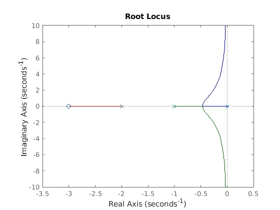
Root locus plot using MATLAB
For loop gain G(s)H(s), we can plot the root locus using the following method:
$$G(s)H(s)=\cfrac{s+3}{s(s+1)(s+2)}$$
num=[1 3];
den=[1 3 2 0];
sys=tf(num,den);
rlocus(sys);
Why we simplify or convert higher-order systems into second-order systems?
Root locus plots can be drawn for a system having lots of roots. However, to understand the meaning of the roots, we try to approximate every higher-order system to a second-order or third-order system. This makes analysis simple.
If it is a third-order system with real coefficients (covers all real systems), it has at least one real root. The other two roots could be a pair of imaginary roots or 2 real roots.
$$1+LG(s)=s^3+as^2+bs+c\hspace{0.5cm}{a,b,c \in{} R}$$
1+LG(s) can be re-written as:
$$1+LG(s)=(s+\alpha{})(s^2+2\zeta{}\omega{}_ns+\omega{}_n^2)\hspace{0.5cm}{\alpha{},\zeta{},\omega{}_n \in{}R}$$
If α is a non-dominant pole, the above third-order system can also be approximated to a second-order system.
Conclusion on root-locus plot
The root locus design technique, created by Walter R. Evans in 1948, is great because it lets designers work directly with the key components (poles and zeros) of a closed-loop system. This means they can control how the system behaves more easily. By placing poles and zeros in the right spots using compensation devices, designers can quickly see how it affects the system's response. Making accurate root locus plots is simple for engineers. However, it works best when you have precise models of the system's components. If these models aren't accurate, the method might not handle uncertainties well.