Analog to Digital converter
An Analog-to-Digital Converter (ADC) is an electronic device or circuit that converts continuous analog signals, such as voltage or current, into discrete digital values. It essentially takes an analog input and converts it into a digital representation that can be processed and manipulated by digital systems, such as microcontrollers, microprocessors, or digital signal processors (DSPs).
Analog to Digital converter calculator
Working principle of an analog to digital converter
Here's how an ADC works:
- Sampling: The first step involves sampling the analog signal at specific time intervals and holding it till the conversion is complete. This process discretizes the continuous analog signal into a series of discrete samples.
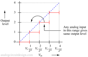
- Quantization: It is the process of mapping the continuous range of sampled analog signals to a finite set of discrete digital values. In other words, it's the process of assigning a specific digital code to each range or level of the analog signal.
- Encoding: The quantized values are encoded into a binary format. Each quantized level corresponds to a specific binary code.
- Output: The binary digital representation of the analog signal is made available as the output of the ADC, which can be processed by a digital system.
$$\text{Digital output code}=\cfrac{\text{Analog input}}{\text{Reference input}}\times{}(2^N-1)$$
Resolution of an ADC or bit-depth
The resolution of an Analog-to-Digital Converter (ADC) is a measure of the ADC's ability to distinguish and represent small changes in an analog input signal. It is defined as the smallest incremental voltage or amplitude change that the ADC can recognize and convert into a change in its digital output.
Resolution is typically expressed in terms of the number of bits in the ADC's digital output. The greater the number of bits, the higher the resolution, as there are more possible digital values to represent the analog signal. For example:
Arduino Uno has a 10-bit ADC that can represent the analog signal with 210 (1024) different digital values, providing 10-bit resolution. If the reference voltage is connected to 5V, the smallest voltage it can measure is 5/1024 = 4.88mV
In practical terms, the resolution of an ADC determines the level of detail or precision with which it can capture and represent the analog signal. A higher-resolution ADC can capture smaller changes in the input signal, making it suitable for applications that require accurate measurements or fine-grained representation of analog data.
Voltage reference of an ADC
The ADC continuously compares the incoming analog signal (often referred to as the "analog input") with the voltage reference. Stability across temperature, stress, and voltage fluctuation is very important. To achieve accuracy, calibration is required sometimes.
Conversion speed of an ADC
The conversion speed in an Analog-to-Digital Converter (ADC) refers to the rate at which the ADC can convert an analog input signal into a digital representation. It is typically measured in terms of samples per second (SPS). Higher conversion speeds are desirable in many applications where you need to sample and digitize rapidly changing analog signals, such as in high-speed data acquisition systems. This conversion speed must be greater than the Nyquist rate (2fs) to avoid aliasing.
Dynamic range of an ADC
The Dynamic range of an ADC is the ratio of the power of highest signal versus the lowest detectable signal. It represents the capability of ADC to detect the lowest signal in presence of high voltage signal without exceeding the overload condition of ADC. Several factors determine the Dynamic range of ADC. Most of them are listed below:
Quantization error and quantisation noise floor
Quantization error refers to the difference between the analog signal and the nearest available digital value at each sampling instance performed by the ADC. This quantization error is responsible for introducing noise, commonly referred to as quantization noise, into the sampled signal. In general, as the resolution of the ADC increases, the quantization error decreases, leading to a reduction in quantization noise.
The relationship between the resolution (expressed in bits) and quantization noise for an ideal ADC can be described as Signal-to-Quantisation-Noise-Ratio (SQNR) :
$$\text{SQNR}=6.02\times{}N+1.76$$
where 'N' represents the ADC's resolution, and SQNR is in decibels (dB). For instance, ideal ADC with different resolutions yields typical SQNR ratios of 72 dB for 12-bit, 60 dB for 10-bit, and 48 dB for 8-bit configurations. This means that, with higher bit resolutions, the signal-to-noise ratio improves, resulting in a more accurate and less noisy representation of the analog signal.
THD (Total harmonic distortion) of an ADC
THD represents the harmonic distortion content of the ADC. It is the ratio of the rms sum of the first six harmonics to the amplitude of the fundamental frequency (of a single frequency sinusoid).
DNL and INL error of an ADC
The DNL (Differential Non-Linearity error) of ith code describes the deviation between two analog values corresponding to adjacent input digital values.
$$\text{DNL}_i=\cfrac{V_{i+1}-V_{i}}{V_{\text{LSB}}}-1$$
The INL (Integral Non-Linearity error) of ith code of an ADC with 2N codes is defined as the absolute value of the difference of the real output voltage minus the ideal expected voltage:
$$\text{INL}_i=|V_{ideal}-V_{real}|$$
SINAD (Signal to Noise and Distortion ratio) of an ADC
SINAD (Signal to Noise and Distortion Ratio) is the ratio of the rms signal amplitude to the mean value of the root-sum-squares (RSS) of all other spectral components including noise and harmonics but excluding DC. SINAD indicates the true usable dynamic range of the ADC.
Effective number of bits (ENOB) of an ADC
The Effective Number of Bits (ENOB) quantifies an ADC's true precision by measuring the equivalent ideal bits it delivers, factoring in noise and distortion. This metric provides a more accurate representation of an ADC's performance compared to its nominal bit count, which can be affected by noise and non-linearity. ENOB is crucial for assessing an ADC's real-world accuracy.
$$\text{ENOB} = (\text{SINAD}-1.76)/6.02$$
Where SINAD is the real world signal to noise and distortion ratio of the ADC.
MSB and LSB of an ADC
- Least significant bit (LSB): The right-most bit in an ADC output code. LSB size is a function of converter resolution. It represents the smallest change that an ADC can detect.
- Most significant bit (MSB): The left-most bit in an ADC output code.
Differential and single ended ADC
- Single-ended ADC - Single-ended ADCs measure a signal relative to a ground reference, making them simple and suitable for single-ended signals with fewer components.
- Differential ADC - Differential-ended ADCs measure the voltage difference between two input signals (termed as positive and negative input terminals), enhancing common mode noise (appearing at both the input terminals) rejection, and are ideal for precise measurements in noisy environments, such as instrumentation and sensors. These are complex to implement but offer better performance.
Types of ADCs
There are several types of ADCs targeting a wide range of applications providing a good cost vs performance tradeoff :
Successive approximation ADC
Successive approximation register (SAR) ADCs operate by iteratively approximating the input analog voltage to a binary digital representation. It starts with setting the MSB as 1. Then compares it with the sampled analog value using a comparator. If the sampled input is less than the digital representation, it will set the bit as 0. Then it moves to the next bit (MSB - 1) and set it 1. This process continues till all bit values are determined. To learn more about please visit this page - Successive approximation ADCs
Flash ADC
A Flash ADC converts analog signals into digital data rapidly (typically within a single cycle). It is known for its high speed but is typically limited in terms of resolution due to its growing architectural complexity at high resolution. The number of comparators required grows exponentially with the desired resolution. This makes them more suitable for applications where speed is crucial, and high resolution is not a primary requirement.
Delta Sigma ADC
Delta-sigma modulation achieves high resolution through a negative feedback loop that continuously corrects quantization errors, effectively suppressing quantization noise in lower frequencies including the signal's bandwidth. A subsequent low-pass filter for demodulation easily eliminates this high-frequency noise and provides accurate amplitude measurements through time averaging. To learn more about Delta-Sigma Modulation, please visit: Delta-Sigma Modulation
Pipeline ADC
A pipeline ADC consists of multiple identical stages, each responsible for a portion of the conversion process. Each stage includes a sample-and-hold circuit, a flash ADC, and digital logic. The first stage samples and holds the present analog input voltage, converts it into some specified digital bits, and passes on the residue to the next stage. The first stage is responsible for the conversion of the analog signal at t=0 while the second stage is responsible for the conversion of sampled value at t=Ts, third stage is responsible for t=2Ts. In a sense, conversion time is still Ts with a delay of NTs, where N is the number of stages in the pipeline ADC.
With pipeline ADCs, a higher resolution can be achieved with a good conversion speed. This is a balance between Flash and SAR ADCs.

Applications of ADCs
- Communication Systems: They digitize voice signals for wireless communication and signal processing in radios.
- Data Acquisition: Used in industrial automation, research, and measurement systems to convert physical parameters like temperature into digital data.
- Audio Processing: Essential for digital audio devices like microphones and speakers.
- Image and Video Processing: Convert light signals in cameras and analog video for digital processing.
- Instrumentation: Precision measurements in oscilloscopes, spectrum analyzers, and more.
- Sensor Interfaces: Convert analog sensor outputs for control and monitoring.
- Wireless and IoT Devices: Used in sensor data acquisition, battery monitoring, and signal processing.
- Medical Equipment: Crucial for ECG machines and blood glucose monitors.
- Radar and Sonar: Digitize signals for target detection in defense and surveillance.
- Automotive Electronics: Control systems, airbags, and sensor measurements.
- Power Monitoring: Manage power quality, grid, and energy metering.
- Environmental Monitoring: Used in air quality, weather, and pollutant sensors.